Getting started with python scripting for MOOSE

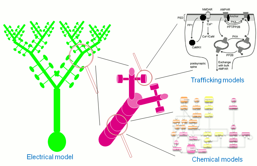
Multiple scales can be modelled and simulated in MOOSE

To see an interactive version of this page, click the following link

This document describes how to use the moose module in Python scripts or in an interactive Python shell. It aims to give you enough overview to help you start scripting using MOOSE and extract farther information that may be required for advanced work. Knowledge of Python or programming in general will be helpful. If you just want to simulate existing models in one of the supported formats, you can fire the MOOSE GUI and locate the model file using the File menu and load it. The GUI is described in separate document. If you are looking for recipes for specific tasks, take a look at cookbook. The example code in the boxes can be entered in a Python shell.

MOOSE is object-oriented. Biological concepts are mapped into classes, and a model is built by creating instances of these classes and connecting them by messages. MOOSE also has numerical classes whose job is to take over difficult computations in a certain domain, and do them fast. There are such solver classes for stochastic and deterministic chemistry, for diffusion, and for multicompartment neuronal models.

MOOSE is a simulation environment, not just a numerical engine: It provides data representations and solvers (of course!), but also a scripting interface with Python, graphical displays with Matplotlib, PyQt, and OpenGL, and support for many model formats. These include SBML, NeuroML, GENESIS kkit and cell.p formats, HDF5 and NSDF for data writing.

Contents:

Coding basics and how to use this document

This page acts as the first stepping stone for learning how moose works. The tutorials here are intended to be interactive, and are presented as python commands. Python commands are identifiable by the >>> before the command as opposed to $ which identifies a command-line command.

>>> this_is_a_python_command

You are encouraged to run a python shell while reading through this documentation and trying out each command for yourself. Python shells are environments within your terminal wherein everything you type is interpreted as a python command. They can be accessed by typing

$ python

in your command-line terminal.

While individually typing lines of code in a python terminal is useful for practicing using moose and coding in general, note that once you close the python environment all the code you typed is gone and the moose models created are also lost. In order to 'save' models that you create, you would have to type your code in a text file with a .py extension. The easiest way to do this is to create a text file in command line, open it with a text editor (for example, gedit), and simply type your code in (make sure you indent correctly).

$ touch code.py
$ gedit code.py

Once you have written your code in the file, you can run it through your python environment.

$ python code.py

Note that apart from this section of the quickstart, most of the moose documentation is in the form of snippets. These are basically .py files with code that demonstrates a certain functionality in moose. If you see a dialogue box like this one:

func.main()

Demonstrate the use of Func class

You can view the code by clicking the green source button on the left side of the box. Alternatively, the source code for all of the examples in the documentation can be found in moose/moose-examples/snippets. Once you run each file in python, it is encouraged that you look through the code to understand how it works.

In the quickstart, most of the snippets demonstrate the functionality of specific classes. However, snippets in later sections such as the cookbook show how to do specific things in moose such as creating networks, chemical models, and synaptic channels.

Importing moose and accessing documentation

In a python script you import modules to access the functionalities they provide. In order to use moose, you need to import it within a python environment or at the beginning of your python script.

>>> import moose

This make the moose module available for use in Python. You can use Python's built-in help function to read the top-level documentation for the moose module.

>>> help(moose)

This will give you an overview of the module. Press q to exit the pager and get back to the interpreter. You can also access the documentation for individual classes and functions this way.

>>> help(moose.connect)

To list the available functions and classes you can use dir function [1].

>>> dir(moose)

MOOSE has built-in documentation in the C++-source-code independent of Python. The moose module has a separate doc function to extract this documentation.

>>> moose.doc('moose.Compartment')

The class level documentation will show whatever the author/maintainer of the class wrote for documentation followed by a list of various kinds of fields and their data types. This can be very useful in an interactive session.

Each field can have its own detailed documentation, too.

>>> moose.doc('Compartment.Rm')

Note that you need to put the class-name followed by dot followed by field-name within quotes. Otherwise, moose.doc will receive the field value as parameter and get confused.

Alternatively, if you want to see a full list of classes, functions and their fields, you can browse through the following pages. This is especially helpful when going through snippets.

• Index
• Module Index

Creating objects and traversing the object hierarchy

Different types of biological entities like neurons, enzymes, etc are represented by classes and individual instances of those types are objects of those classes. Objects are the building-blocks of models in MOOSE. We call MOOSE objects element and use object and element interchangeably in the context of MOOSE. Elements are conceptually laid out in a tree-like hierarchical structure. If you are familiar with file system hierarchies in common operating systems, this should be simple.

At the top of the object hierarchy sits the Shell, equivalent to the root directory in UNIX-based systems and represented by the path /. You can list the existing objects under / using the le function.

>>> moose.le()
Elements under /
/Msgs
/clock
/classes
/postmaster

Msgs, clock and classes are predefined objects in MOOSE. And each object can contain other objects inside them. You can see them by passing the path of the parent object to le

>>> moose.le('/Msgs')
Elements under /Msgs[0]
/Msgs[0]/singleMsg
/Msgs[0]/oneToOneMsg
/Msgs[0]/oneToAllMsg
/Msgs[0]/diagonalMsg
/Msgs[0]/sparseMsg

Now let us create some objects of our own. This can be done by invoking MOOSE class constructors (just like regular Python classes).

>>> model = moose.Neutral('/model')

The above creates a Neutral object named model. Neutral is the most basic class in MOOSE. A Neutral element can act as a container for other elements. We can create something under model

>>> soma = moose.Compartment('/model/soma')

Every element has a unique path. This is a concatenation of the names of all the objects one has to traverse starting with the root to reach that element.

>>> print soma.path
/model/soma

The name of the element can be printed, too.

>>> print soma.name
soma

The Compartment elements model small sections of a neuron. Some basic experiments can be carried out using a single compartment. Let us create another object to act on the soma. This will be a step current generator to inject a current pulse into the soma.

>>> pulse = moose.PulseGen('/model/pulse')

You can use le at any point to see what is there

>>> moose.le('/model')
Elements under /model
/model/soma
/model/pulse

And finally, we can create a Table to record the time series of the soma's membrane potential. It is good practice to organize the data separately from the model. So we do it as below

>>> data = moose.Neutral('/data')
>>> vmtab = moose.Table('/data/soma_Vm')

Now that we have the essential elements for a small model, we can go on to set the properties of this model and the experimental protocol.

Setting the properties of elements: accessing fields

Elements have several kinds of fields. The simplest ones are the value fields. These can be accessed like ordinary Python members. You can list the available value fields using getFieldNames function

>>> soma.getFieldNames('valueFinfo')

Here valueFinfo is the type name for value fields. Finfo is short form of field information. For each type of field there is a name ending with -Finfo. The above will display the following list

 ('this',
'name',
'me',
'parent',
'children',
'path',
'class',
'linearSize',
'objectDimensions',
'lastDimension',
'localNumField',
'pathIndices',
'msgOut',
'msgIn',
'Vm',
'Cm',
'Em',
'Im',
'inject',
'initVm',
'Rm',
'Ra',
'diameter',
'length',
'x0',
'y0',
'z0',
'x',
'y',
'z')

Some of these fields are for internal or advanced use, some give access to the physical properties of the biological entity we are trying to model. Now we are interested in Cm, Rm, Em and initVm. In the most basic form, a neuronal compartment acts like a parallel RC circuit with a battery attached. Here R and C are resistor and capacitor connected in parallel, and the battery with voltage Em is in series with the resistor, as shown below:

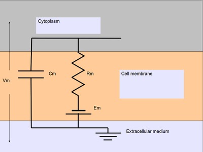
Passive neuronal compartment

The fields are populated with some defaults.

>>> print soma.Cm, soma.Rm, soma.Vm, soma.Em, soma.initVm
1.0 1.0 -0.06 -0.06 -0.06

You can set the Cm and Rm fields to something realistic using simple assignment (we follow SI unit) [2].

>>> soma.Cm = 1e-9
>>> soma.Rm = 1e7
>>> soma.initVm = -0.07

Instead of writing print statements for each field, you could use the utility function showfield to see that the changes took effect

>>> moose.showfield(soma)
[ /soma[0] ]
diameter         = 0.0
Ra               = 1.0
y0               = 0.0
Rm               = 10000000.0
numData          = 1
inject           = 0.0
initVm           = -0.07
Em               = -0.06
y                = 0.0
numField         = 1
path             = /soma[0]
dt               = 5e-05
tick             = 4
z0               = 0.0
name             = soma
Cm               = 1e-09
x0               = 0.0
Vm               = -0.06
className        = Compartment
length           = 0.0
Im               = 0.0
x                = 0.0
z                = 0.0

Now we can setup the current pulse to be delivered to the soma

>>> pulse.delay[0] = 50e-3
>>> pulse.width[0] = 100e-3
>>> pulse.level[0] = 1e-9
>>> pulse.delay[1] = 1e9

This tells the pulse generator to create a 100 ms long pulse 50 ms after the start of the simulation. The amplitude of the pulse is set to 1 nA. We set the delay for the next pulse to a very large value (larger than the total simulation time) so that the stimulation stops after the first pulse. Had we set pulse.delay = 0 , it would have generated a pulse train at 50 ms intervals.

Putting them together: setting up connections

In order for the elements to interact during simulation, we need to connect them via messages. Elements are connected to each other using special source and destination fields. These types are named srcFinfo and destFinfo. You can query the available source and destination fields on an element using getFieldNames as before. This time, let us do it another way: by the class name

>>> moose.getFieldNames('PulseGen', 'srcFinfo')
('childMsg', 'output')

This form has the advantage that you can get information about a class without creating elements of that class.

Here childMsg is a source field that is used by the MOOSE internals to connect child elements to parent elements. The second one is of our interest. Check out the built-in documentation here

>>> moose.doc('PulseGen.output')
PulseGen.output: double - source field
Current output level.

so this is the output of the pulse generator and this must be injected into the soma to stimulate it. But where in the soma can we send it? Again, MOOSE has some introspection built in.

>>> soma.getFieldNames('destFinfo')
('parentMsg',
 'setThis',
 'getThis',
   ...
 'setZ',
 'getZ',
 'injectMsg',
 'randInject',
 'cable',
 'process',
 'reinit',
 'initProc',
 'initReinit',
 'handleChannel',
 'handleRaxial',
 'handleAxial')

Now that is a long list. But much of it are fields for internal or special use. Anything that starts with get or set are internal destFinfo used for accessing value fields (we shall use one of those when setting up data recording). Among the rest injectMsg seems to be the most likely candidate. Use the connect function to connect the pulse generator output to the soma input

>>> m = moose.connect(pulse, 'output', soma, 'injectMsg')

connect(source, source_field, dest, dest_field) creates a message from source element's source_field field to dest element's dest_field field and returns that message. Messages are also elements. You can print them to see their identity

>>> print m
<moose.SingleMsg: id=5, dataId=733, path=/Msgs/singleMsg[733]>

You can print any element as above and the string representation will show you the class, two numbers(id and dataId) uniquely identifying it among all elements, and its path. You can get some more information about a message

>>> print m.e1.path, m.e2.path, m.srcFieldsOnE1, m.destFieldsOnE2
/model/pulse /model/soma ('output',) ('injectMsg',)

will confirm what you already know.

A message element has fields e1 and e2 referring to the elements it connects. For single one-directional messages these are source and destination elements, which are pulse and soma respectively. The next two items are lists of the field names which are connected by this message.

You could also check which elements are connected to a particular field

>>> print soma.neighbors['injectMsg']
[<moose.vec: class=PulseGen, id=729,path=/model/pulse>]

Notice that the list contains something called vec. We discuss this later. Also neighbors is a new kind of field: lookupFinfo which behaves like a dictionary. Next we connect the table to the soma to retrieve its membrane potential Vm. This is where all those destFinfo starting with get or set come in use. For each value field X, there is a destFinfo get{X} to retrieve the value at simulation time. This is used by the table to record the values Vm takes.

>>> moose.connect(vmtab, 'requestOut', soma, 'getVm')
<moose.SingleMsg: id=5, dataIndex=0, path=/Msgs[0]/singleMsg[0]>

This finishes our model and recording setup. You might be wondering about the source-destination relationship above. It is natural to think that soma is the source of Vm values which should be sent to vmtab. But here requestOut is a srcFinfo acting like a reply card. This mode of obtaining data is called pull mode. [3]

You can skip the next section on fine control of the timing of updates and read Running the simulation.

Scheduling

With the model all set up, we have to schedule the simulation. Different components in a model may have different rates of update. For example, the dynamics of electrical components require the update intervals to be of the order 0.01 ms whereas chemical components can be as slow as 1 s. Also, the results may depend on the sequence of the updates of different components. These issues are addressed in MOOSE using a clock-based update scheme. Each model component is scheduled on a clock tick (think of multiple hands of a clock ticking at different intervals and the object being updated at each tick of the corresponding hand). The scheduling also guarantees the correct sequencing of operations. For example, your Table objects should always be scheduled after the computations that they are recording, otherwise they will miss the outcome of the latest calculation.

MOOSE has a central clock element (/clock) to manage time. Clock has a set of Tick elements under it that take care of advancing the state of each element with time as the simulation progresses. Every element to be included in a simulation must be assigned a tick. Each tick can have a different ticking interval (dt) that allows different elements to be updated at different rates.

By default, every object is assigned a clock tick with reasonable default timesteps as soon it is created:

Class type                      tick    dt
Electrical computations:        0-7     50 microseconds
electrical compartments,
V and ligand-gated ion channels,
Calcium conc and Nernst,
stimulus generators and tables,
HSolve.

Table (to plot elec. signals)   8       100 microseconds

Diffusion solver                10      0.01 seconds
Chemical computations:          11-17   0.1 seconds
Pool, Reac, Enz, MMEnz,
Func, Function,
Gsolve, Ksolve,
Stats (to do stats on outputs)

Table2 (to plot chem. signals)  18      1 second

HDF5DataWriter                  30      1 second
Postmaster (for parallel        31      0.01 seconds
computations)

There are 32 available clock ticks. Numbers 20 to 29 are unassigned so you can use them for whatever purpose you like.

If you want fine control over the scheduling, there are three things you can do.

• Alter the 'tick' field on the object
• Alter the dt associated with a given tick, using the moose.setClock( tick, newdt) command
• Go through a wildcard path of objects reassigning there clock ticks, using moose.useClock( path, newtick, function).

Here we discuss these in more detail.

Altering the 'tick' field

Every object knows which tick and dt it uses:

>>> a = moose.Pool( '/a' )
>>> print a.tick, a.dt
13 0.1

The tick field on every object can be changed, and the object will adopt whatever clock dt is used for that tick. The dt field is readonly, because changing it would have side-effects on every object associated with the current tick.

Ticks -1 and -2 are special: They both tell the object that it is disabled (not scheduled for any operations). An object with a tick of -1 will be left alone entirely. A tick of -2 is used in solvers to indicate that should the solver be removed, the object will revert to its default tick.

Altering the dt associated with a given tick

We initialize the ticks and set their dt values using the setClock function.

>>> moose.setClock(0, 0.025e-3)
>>> moose.setClock(1, 0.025e-3)
>>> moose.setClock(2, 0.25e-3)

This will initialize tick #0 and tick #1 with dt = 25 μs and tick #2 with dt = 250 μs. Thus all the elements scheduled on ticks #0 and 1 will be updated every 25 μs and those on tick #2 every 250 μs. We use the faster clocks for the model components where finer timescale is required for numerical accuracy and the slower clock to sample the values of Vm.

Note that if you alter the dt associated with a given tick, this will affect the update time for all the objects using that clock tick. If you're unsure that you want to do this, use one of the vacant ticks.

Assigning clock ticks to all objects in a wildcard path

To assign tick #2 to the table for recording Vm, we pass its whole path to the useClock function.

>>> moose.useClock(2, '/data/soma_Vm', 'process')

Read this as "use tick # 2 on the element at path /data/soma_Vm to call its process method at every step". Every class that is supposed to update its state or take some action during simulation implements a process method. And in most cases that is the method we want the ticks to call at every time step. A less common method is init, which is implemented in some classes to interleave actions or updates that must be executed in a specific order [4]. The Compartment class is one such case where a neuronal compartment has to know the Vm of its neighboring compartments before it can calculate its Vm for the next step. This is done with:

>>> moose.useClock(0, soma.path, 'init')

Here we used the path field instead of writing the path explicitly.

Next we assign tick #1 to process method of everything under /model.

>>> moose.useClock(1, '/model/##', 'process')

Here the second argument is an example of wild-card path. The ## matches everything under the path preceding it at any depth. Thus if we had some other objects under /model/soma, process method of those would also have been scheduled on tick #1. This is very useful for complex models where it is tedious to scheduled each element individually. In this case we could have used /model/# as well for the path. This is a single level wild-card which matches only the children of /model but does not go farther down in the hierarchy.

Running the simulation

Once the model is all set up, we can put the model to its initial state using

>>> moose.reinit()

You may remember that we had changed initVm from -0.06 to -0.07. The reinit call we initialize Vm to that value. You can verify that

>>> print soma.Vm
-0.07

Finally, we run the simulation for 300 ms

>>> moose.start(300e-3)

The data will be recorded by the soma_vm table, which is referenced by the variable vmtab. The Table class provides a numpy array interface to its content. The field is vector. So you can easily plot the membrane potential using the matplotlib library.

>>> import pylab
>>> t = pylab.linspace(0, 300e-3, len(vmtab.vector))
>>> pylab.plot(t, vmtab.vector)
>>> pylab.show()

The first line imports the pylab submodule from matplotlib. This useful for interactive plotting. The second line creates the time points to match our simulation time and length of the recorded data. The third line plots the Vm and the fourth line makes it visible. Does the plot match your expectation?

Some more details

vec, melement and element

MOOSE elements are instances of the class melement. Compartment, PulseGen and other MOOSE classes are derived classes of melement. All melement instances are contained in array-like structures called vec. Each vec object has a numerical id_ field uniquely identifying it. An vec can have one or more elements. You can create an array of elements

>>> comp_array = moose.vec('/model/comp', n=3, dtype='Compartment')

This tells MOOSE to create an vec of 3 Compartment elements with path /model/comp. For vec objects with multiple elements, the index in the vec is part of the element path.

>>> print comp_array.path, type(comp_array)

shows that comp_array is an instance of vec class. You can loop through the elements in an vec like a Python list

>>> for comp in comp_array:
...    print comp.path, type(comp)
...

shows

/model[0]/comp[0] <type 'moose.Compartment'>
/model[0]/comp[1] <type 'moose.Compartment'>
/model[0]/comp[2] <type 'moose.Compartment'>

Thus elements are instances of class melement. All elements in an vec share the id_ of the vec which can retrieved by melement.getId().

A frequent use case is that after loading a model from a file one knows the paths of various model components but does not know the appropriate class name for them. For this scenario there is a function called element which converts ("casts" in programming jargon) a path or any moose object to its proper MOOSE class. You can create additional references to soma in the example this way

x = moose.element('/model/soma')

Any MOOSE class can be extended in Python. But any additional attributes added in Python are invisible to MOOSE. So those can be used for functionalities at the Python level only. You can see moose-examples/squid/squid.py for an example.

Finfos

The following kinds of Finfo are accessible in Python

• ``valueFinfo`` : simple values. For each readable valueFinfo XYZ there is a destFinfo getXYZ that can be used for reading the value at run time. If XYZ is writable then there will also be destFinfo to set it: setXYZ. Example: Compartment.Rm
• ``lookupFinfo`` : lookup tables. These fields act like Python dictionaries but iteration is not supported. Example: Neutral.neighbors.
• ``srcFinfo`` : source of a message. Example: PulseGen.output.
• ``destFinfo`` : destination of a message. Example: Compartment.injectMsg. Apart from being used in setting up messages, these are accessible as functions from Python. HHGate.setupAlpha is an example.
• ``sharedFinfo`` : a composition of source and destination fields. Example: Compartment.channel.

Moving on

Now you know the basics of pymoose and how to access the help system. You can figure out how to do specific things by looking at the 'cookbook`. In addition, the moose-examples/snippets directory in your MOOSE installation has small executable python scripts that show usage of specific classes or functionalities. Beyond that you can browse the code in the moose-examples directory to see some more complex models.

MOOSE is backward compatible with GENESIS and most GENESIS classes have been reimplemented in MOOSE. There is slight change in naming (MOOSE uses CamelCase), and setting up messages are different. But GENESIS documentation is still a good source for documentation on classes that have been ported from GENESIS.

If the built-in MOOSE classes do not satisfy your needs entirely, you are welcome to add new classes to MOOSE. The API documentation will help you get started.

[1]	To list the classes only, use moose.le('/classes')

[2]	MOOSE is unit agnostic and things should work fine as long as you use values all converted to a consistent unit system.

[3]	This apparently convoluted implementation is for performance reason. Can you figure out why? Hint: the table is driven by a slower clock than the compartment.

[4]	In principle any function available in a MOOSE class can be executed periodically this way as long as that class exposes the function for scheduling following the MOOSE API. So you have to consult the class' documentation for any nonstandard methods that can be scheduled this way.