Chemical Bistables
A bistable system is a dynamic system that has two stable equilibrium states. The following examples can be used to teach and demonstrate different aspects of bistable systems or to learn how to model them using moose. Each example contains a short description, the model's code, and the output with default settings.
Each example can be found as a python file within the main moose folder under
(...)/moose/moose-examples/tutorials/ChemicalBistables
In order to run the example, run the script
in command line, where filename.py is the name of the python file you would like to run. The filenames of each example are written in bold at the beginning of their respective sections, and the files themselves can be found in the aformentioned directory.
In chemical bistable models that use solvers, there are optional arguments that allow you to specify which solver you would like to use.
python filename.py [gsl | gssa | ee]
Where:
- gsl: This is the Runge-Kutta-Fehlberg implementation from the GNU Scientific Library (GSL). It is a fifth order variable timestep explicit method. Works well for most reaction systems except if they have very stiff reactions.
- gssl: Optimized Gillespie stochastic systems algorithm, custom implementation. This uses variable timesteps internally. Note that it slows down with increasing numbers of molecules in each pool. It also slows down, but not so badly, if the number of reactions goes up.
- Exponential Euler:This methods computes the solution of partial and ordinary differential equations.
All the following examples can be run with either of the three solvers, each of which has different advantages and disadvantages and each of which might produce a slightly different outcome.
Simply running the file without the optional argument will by default use the gsl solver. These gsl outputs are the ones shown below.
Simple Bistables
Filename: simpleBis.py
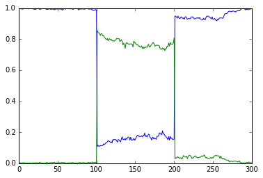
This example shows the key property of a chemical bistable system: it
has two stable states. Here we start out with the system settling rather
quickly to the first stable state, where molecule A is high (blue) and
the complementary molecule B (green) is low. At t = 100s, we deliver a
perturbation, which is to move 90% of the A molecules into B. This
triggers a state flip, which settles into a distinct stable state where
there is more of B than of A. At t = 200s we reverse the flip by moving
99% of B molecules back to A.
If we run the simulation with the gssa option python simpleBis.py gssa
we see exactly the same sequence of events, except now the switch is
noisy. The calculations are now run with the Gillespie Stochastic
Systems Algorithm (gssa) which incorporates probabilistic reaction
events. The switch still switches but one can see that it might flip
spontaneously once in a while.
Things to do:
1. Open a copy of the script file in an editor, and around
line 124 and 129 you will see how the state flip is implemented while
maintaining mass conservation. What happens if you flip over fewer
molecules? What is the threshold for a successful flip? Why are these
thresholds different for the different states?
- Try different volumes in line 31, and rerun using the gssa. Will you
see more or less noise if you increase the volume to 1e-20 m^3?
Code:
Show/Hide code 1
2
3
4
5
6
7
8
9
10
11
12
13
14
15
16
17
18
19
20
21
22
23
24
25
26
27
28
29
30
31
32
33
34
35
36
37
38
39
40
41
42
43
44
45
46
47
48
49
50
51
52
53
54
55
56
57
58
59
60
61
62
63
64
65
66
67
68
69
70
71
72
73
74
75
76
77
78
79
80
81
82
83
84
85
86
87
88
89
90
91
92
93
94
95
96
97
98
99
100
101
102
103
104
105
106
107
108
109
110
111
112
113
114
115
116
117
118
119
120
121
122
123
124
125
126
127
128
129
130
131
132
133
134
135
136
137
138
139
140 | #########################################################################
## This program is part of 'MOOSE', the
## Messaging Object Oriented Simulation Environment.
## Copyright (C) 2013 Upinder S. Bhalla. and NCBS
## It is made available under the terms of the
## GNU Lesser General Public License version 2.1
## See the file COPYING.LIB for the full notice.
#########################################################################
# This example illustrates how to set up a kinetic solver and kinetic model
# using the scripting interface. Normally this would be done using the
# Shell::doLoadModel command, and normally would be coordinated by the
# SimManager as the base of the entire model.
# This example creates a bistable model having two enzymes and a reaction.
# One of the enzymes is autocatalytic.
# The model is set up to run using deterministic integration.
# If you pass in the argument 'gssa' it will run with the stochastic
# solver instead
# You may also find it interesting to change the volume.
import math
import pylab
import numpy
import moose
import sys
def makeModel():
# create container for model
model = moose.Neutral( 'model' )
compartment = moose.CubeMesh( '/model/compartment' )
compartment.volume = 1e-21 # m^3
# the mesh is created automatically by the compartment
mesh = moose.element( '/model/compartment/mesh' )
# create molecules and reactions
a = moose.Pool( '/model/compartment/a' )
b = moose.Pool( '/model/compartment/b' )
c = moose.Pool( '/model/compartment/c' )
enz1 = moose.Enz( '/model/compartment/b/enz1' )
enz2 = moose.Enz( '/model/compartment/c/enz2' )
cplx1 = moose.Pool( '/model/compartment/b/enz1/cplx' )
cplx2 = moose.Pool( '/model/compartment/c/enz2/cplx' )
reac = moose.Reac( '/model/compartment/reac' )
# connect them up for reactions
moose.connect( enz1, 'sub', a, 'reac' )
moose.connect( enz1, 'prd', b, 'reac' )
moose.connect( enz1, 'enz', b, 'reac' )
moose.connect( enz1, 'cplx', cplx1, 'reac' )
moose.connect( enz2, 'sub', b, 'reac' )
moose.connect( enz2, 'prd', a, 'reac' )
moose.connect( enz2, 'enz', c, 'reac' )
moose.connect( enz2, 'cplx', cplx2, 'reac' )
moose.connect( reac, 'sub', a, 'reac' )
moose.connect( reac, 'prd', b, 'reac' )
# connect them up to the compartment for volumes
#for x in ( a, b, c, cplx1, cplx2 ):
# moose.connect( x, 'mesh', mesh, 'mesh' )
# Assign parameters
a.concInit = 1
b.concInit = 0
c.concInit = 0.01
enz1.kcat = 0.4
enz1.Km = 4
enz2.kcat = 0.6
enz2.Km = 0.01
reac.Kf = 0.001
reac.Kb = 0.01
# Create the output tables
graphs = moose.Neutral( '/model/graphs' )
outputA = moose.Table ( '/model/graphs/concA' )
outputB = moose.Table ( '/model/graphs/concB' )
# connect up the tables
moose.connect( outputA, 'requestOut', a, 'getConc' );
moose.connect( outputB, 'requestOut', b, 'getConc' );
# Schedule the whole lot
moose.setClock( 4, 0.01 ) # for the computational objects
moose.setClock( 8, 1.0 ) # for the plots
# The wildcard uses # for single level, and ## for recursive.
moose.useClock( 4, '/model/compartment/##', 'process' )
moose.useClock( 8, '/model/graphs/#', 'process' )
def displayPlots():
for x in moose.wildcardFind( '/model/graphs/conc#' ):
t = numpy.arange( 0, x.vector.size, 1 ) #sec
pylab.plot( t, x.vector, label=x.name )
pylab.legend()
pylab.show()
def main():
solver = "gsl"
makeModel()
if ( len ( sys.argv ) == 2 ):
solver = sys.argv[1]
stoich = moose.Stoich( '/model/compartment/stoich' )
stoich.compartment = moose.element( '/model/compartment' )
if ( solver == 'gssa' ):
gsolve = moose.Gsolve( '/model/compartment/ksolve' )
stoich.ksolve = gsolve
else:
ksolve = moose.Ksolve( '/model/compartment/ksolve' )
stoich.ksolve = ksolve
stoich.path = "/model/compartment/##"
#solver.method = "rk5"
#mesh = moose.element( "/model/compartment/mesh" )
#moose.connect( mesh, "remesh", solver, "remesh" )
moose.setClock( 5, 1.0 ) # clock for the solver
moose.useClock( 5, '/model/compartment/ksolve', 'process' )
moose.reinit()
moose.start( 100.0 ) # Run the model for 100 seconds.
a = moose.element( '/model/compartment/a' )
b = moose.element( '/model/compartment/b' )
# move most molecules over to b
b.conc = b.conc + a.conc * 0.9
a.conc = a.conc * 0.1
moose.start( 100.0 ) # Run the model for 100 seconds.
# move most molecules back to a
a.conc = a.conc + b.conc * 0.99
b.conc = b.conc * 0.01
moose.start( 100.0 ) # Run the model for 100 seconds.
# Iterate through all plots, dump their contents to data.plot.
displayPlots()
quit()
# Run the 'main' if this script is executed standalone.
if __name__ == '__main__':
main()
|
Output:
Scale Volumes
File name: scaleVolumes.py
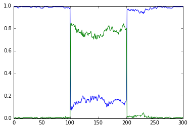
This script runs exactly the same model as in simpleBis.py, but it
automatically scales the volumes from 1e-19 down to smaller values.
Note how the simulation successively becomes noisier, until at very
small volumes there are spontaneous state transitions.
Code:
Show/Hide code 1
2
3
4
5
6
7
8
9
10
11
12
13
14
15
16
17
18
19
20
21
22
23
24
25
26
27
28
29
30
31
32
33
34
35
36
37
38
39
40
41
42
43
44
45
46
47
48
49
50
51
52
53
54
55
56
57
58
59
60
61
62
63
64
65
66
67
68
69
70
71
72
73
74
75
76
77
78
79
80
81
82
83
84
85
86
87
88
89
90
91
92
93
94
95
96
97
98
99
100
101
102
103
104
105
106
107
108
109
110
111
112
113
114
115
116
117
118
119
120
121
122
123
124
125
126
127
128
129
130
131
132
133
134
135
136
137
138
139
140
141
142
143
144
145
146
147
148
149
150
151
152
153
154
155
156 | #########################################################################
## This program is part of 'MOOSE', the
## Messaging Object Oriented Simulation Environment.
## Copyright (C) 2013 Upinder S. Bhalla. and NCBS
## It is made available under the terms of the
## GNU Lesser General Public License version 2.1
## See the file COPYING.LIB for the full notice.
#########################################################################
import math
import pylab
import numpy
import moose
def makeModel():
# create container for model
model = moose.Neutral( 'model' )
compartment = moose.CubeMesh( '/model/compartment' )
compartment.volume = 1e-20
# the mesh is created automatically by the compartment
mesh = moose.element( '/model/compartment/mesh' )
# create molecules and reactions
a = moose.Pool( '/model/compartment/a' )
b = moose.Pool( '/model/compartment/b' )
c = moose.Pool( '/model/compartment/c' )
enz1 = moose.Enz( '/model/compartment/b/enz1' )
enz2 = moose.Enz( '/model/compartment/c/enz2' )
cplx1 = moose.Pool( '/model/compartment/b/enz1/cplx' )
cplx2 = moose.Pool( '/model/compartment/c/enz2/cplx' )
reac = moose.Reac( '/model/compartment/reac' )
# connect them up for reactions
moose.connect( enz1, 'sub', a, 'reac' )
moose.connect( enz1, 'prd', b, 'reac' )
moose.connect( enz1, 'enz', b, 'reac' )
moose.connect( enz1, 'cplx', cplx1, 'reac' )
moose.connect( enz2, 'sub', b, 'reac' )
moose.connect( enz2, 'prd', a, 'reac' )
moose.connect( enz2, 'enz', c, 'reac' )
moose.connect( enz2, 'cplx', cplx2, 'reac' )
moose.connect( reac, 'sub', a, 'reac' )
moose.connect( reac, 'prd', b, 'reac' )
# connect them up to the compartment for volumes
#for x in ( a, b, c, cplx1, cplx2 ):
# moose.connect( x, 'mesh', mesh, 'mesh' )
# Assign parameters
a.concInit = 1
b.concInit = 0
c.concInit = 0.01
enz1.kcat = 0.4
enz1.Km = 4
enz2.kcat = 0.6
enz2.Km = 0.01
reac.Kf = 0.001
reac.Kb = 0.01
# Create the output tables
graphs = moose.Neutral( '/model/graphs' )
outputA = moose.Table ( '/model/graphs/concA' )
outputB = moose.Table ( '/model/graphs/concB' )
# connect up the tables
moose.connect( outputA, 'requestOut', a, 'getConc' );
moose.connect( outputB, 'requestOut', b, 'getConc' );
# Schedule the whole lot
moose.setClock( 4, 0.01 ) # for the computational objects
moose.setClock( 8, 1.0 ) # for the plots
# The wildcard uses # for single level, and ## for recursive.
moose.useClock( 4, '/model/compartment/##', 'process' )
moose.useClock( 8, '/model/graphs/#', 'process' )
def displayPlots():
for x in moose.wildcardFind( '/model/graphs/conc#' ):
t = numpy.arange( 0, x.vector.size, 1 ) #sec
pylab.plot( t, x.vector, label=x.name )
def main():
"""
This example illustrates how to run a model at different volumes.
The key line is just to set the volume of the compartment::
compt.volume = vol
If everything
else is set up correctly, then this change propagates through to all
reactions molecules.
For a deterministic reaction one would not see any change in output
concentrations.
For a stochastic reaction illustrated here, one sees the level of
'noise'
changing, even though the concentrations are similar up to a point.
This example creates a bistable model having two enzymes and a reaction.
One of the enzymes is autocatalytic.
This model is set up within the script rather than using an external
file.
The model is set up to run using the GSSA (Gillespie Stocahstic systems
algorithim) method in MOOSE.
To run the example, run the script
``python scaleVolumes.py``
and close the plots every cycle to see the outcome of stochastic
calculations at ever smaller volumes, keeping concentrations the same.
"""
makeModel()
moose.seed( 11111 )
gsolve = moose.Gsolve( '/model/compartment/gsolve' )
stoich = moose.Stoich( '/model/compartment/stoich' )
compt = moose.element( '/model/compartment' );
stoich.compartment = compt
stoich.ksolve = gsolve
stoich.path = "/model/compartment/##"
moose.setClock( 5, 1.0 ) # clock for the solver
moose.useClock( 5, '/model/compartment/gsolve', 'process' )
a = moose.element( '/model/compartment/a' )
for vol in ( 1e-19, 1e-20, 1e-21, 3e-22, 1e-22, 3e-23, 1e-23 ):
# Set the volume
compt.volume = vol
print('vol = {}, a.concInit = {}, a.nInit = {}'.format( vol, a.concInit, a.nInit))
print('Close graph to go to next plot\n')
moose.reinit()
moose.start( 100.0 ) # Run the model for 100 seconds.
a = moose.element( '/model/compartment/a' )
b = moose.element( '/model/compartment/b' )
# move most molecules over to b
b.conc = b.conc + a.conc * 0.9
a.conc = a.conc * 0.1
moose.start( 100.0 ) # Run the model for 100 seconds.
# move most molecules back to a
a.conc = a.conc + b.conc * 0.99
b.conc = b.conc * 0.01
moose.start( 100.0 ) # Run the model for 100 seconds.
# Iterate through all plots, dump their contents to data.plot.
displayPlots()
pylab.show()
quit()
# Run the 'main' if this script is executed standalone.
if __name__ == '__main__':
main()
|
Output:
vol = 1e-19, a.concInit = 1.0, a.nInit = 60221.415
vol = 1e-20, a.concInit = 1.0, a.nInit = 6022.1415
vol = 1e-21, a.concInit = 1.0, a.nInit = 602.21415
vol = 3e-22, a.concInit = 1.0, a.nInit = 180.664245
vol = 1e-22, a.concInit = 1.0, a.nInit = 60.221415
vol = 3e-23, a.concInit = 1.0, a.nInit = 18.0664245
vol = 1e-23, a.concInit = 1.0, a.nInit = 6.0221415
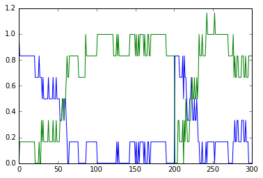
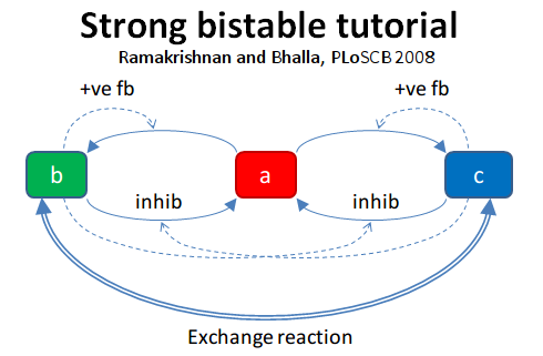
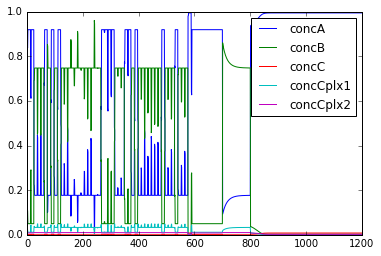
Strong Bistable System
File name: strongBis.py
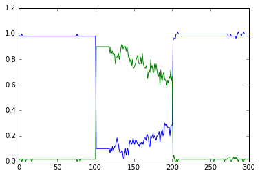
This example illustrates a particularly strong, that is, parametrically
robust bistable system. The model topology is symmetric between
molecules b and c. We have both positive feedback of molecules
b and c onto themselves, and also inhibition of b by c
and vice versa.
Open the python file to see what is happening. The simulation starts at
a symmetric point and the model settles at precisely the balance point
where a, b, and c are at the same concentration. At t= 100
we apply a small molecular 'tap' to push it over to a state where c
is larger. This is stable. At t = 210 we apply a moderate push to show
that it is now very stably in this state, and the system rebounds to its
original levels. At t = 320 we apply a strong push to take it over to a
state where b is larger. At t = 430 we give it a strong push to take
it back to the c dominant state.
Code:
Show/Hide code 1
2
3
4
5
6
7
8
9
10
11
12
13
14
15
16
17
18
19
20
21
22
23
24
25
26
27
28
29
30
31
32
33
34
35
36
37
38
39
40
41
42
43
44
45
46
47
48
49
50
51
52
53
54
55
56
57
58
59
60
61
62
63
64
65
66
67
68
69
70
71
72
73
74 | #########################################################################
## This program is part of 'MOOSE', the
## Messaging Object Oriented Simulation Environment.
## Copyright (C) 2014 Upinder S. Bhalla. and NCBS
## It is made available under the terms of the
## GNU Lesser General Public License version 2.1
## See the file COPYING.LIB for the full notice.
#########################################################################
import moose
import matplotlib.pyplot as plt
import matplotlib.image as mpimg
import pylab
import numpy
import sys
def main():
solver = "gsl" # Pick any of gsl, gssa, ee..
#solver = "gssa" # Pick any of gsl, gssa, ee..
#moose.seed( 1234 ) # Needed if stochastic.
mfile = '../../genesis/M1719.g'
runtime = 100.0
if ( len( sys.argv ) >= 2 ):
solver = sys.argv[1]
modelId = moose.loadModel( mfile, 'model', solver )
# Increase volume so that the stochastic solver gssa
# gives an interesting output
compt = moose.element( '/model/kinetics' )
compt.volume = 0.2e-19
r = moose.element( '/model/kinetics/equil' )
moose.reinit()
moose.start( runtime )
r.Kf *= 1.1 # small tap to break symmetry
moose.start( runtime/10 )
r.Kf = r.Kb
moose.start( runtime )
r.Kb *= 2.0 # Moderate push does not tip it back.
moose.start( runtime/10 )
r.Kb = r.Kf
moose.start( runtime )
r.Kb *= 5.0 # Strong push does tip it over
moose.start( runtime/10 )
r.Kb = r.Kf
moose.start( runtime )
r.Kf *= 5.0 # Strong push tips it back.
moose.start( runtime/10 )
r.Kf = r.Kb
moose.start( runtime )
# Display all plots.
img = mpimg.imread( 'strongBis.png' )
fig = plt.figure( figsize=(12, 10 ) )
png = fig.add_subplot( 211 )
imgplot = plt.imshow( img )
ax = fig.add_subplot( 212 )
x = moose.wildcardFind( '/model/#graphs/conc#/#' )
dt = moose.element( '/clock' ).tickDt[18]
t = numpy.arange( 0, x[0].vector.size, 1 ) * dt
ax.plot( t, x[0].vector, 'r-', label=x[0].name )
ax.plot( t, x[1].vector, 'g-', label=x[1].name )
ax.plot( t, x[2].vector, 'b-', label=x[2].name )
plt.ylabel( 'Conc (mM)' )
plt.xlabel( 'Time (seconds)' )
pylab.legend()
pylab.show()
# Run the 'main' if this script is executed standalone.
if __name__ == '__main__':
main()
|
Output:
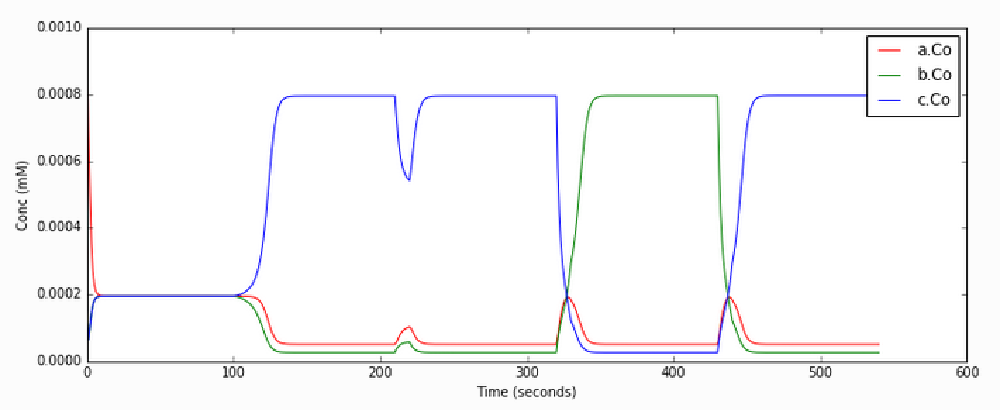
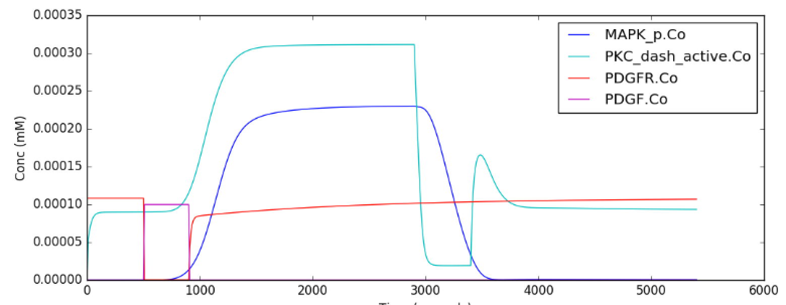
MAPK Feedback Model
File name: mapkFB.py
This example illustrates loading, and running a kinetic model for a much
more complex bistable positive feedback system, defined in kkit format.
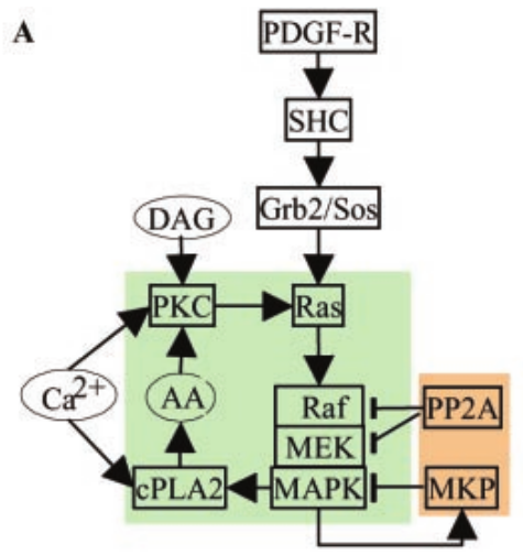
This is based on Bhalla, Ram and Iyengar, Science 2002.
The core of this model is a positive feedback loop comprising of the
MAPK cascade, PLA2, and PKC. It receives PDGF and Ca2+ as inputs.
This model is quite a large one and due to some stiffness in its
equations, it takes about 30 seconds to execute. Note that this is still
200 times faster than the events it models.
The simulation illustrated here shows how the model starts out in a
state of low activity. It is induced to 'turn on' when a a PDGF stimulus
is given for 400 seconds, starting at t = 500s. After it has settled to
the new 'on' state, the model is made to 'turn off' by setting the
system calcium levels to zero. This inhibition starts at t = 2900 and
goes on for 500 s.
Note that this is a somewhat unphysiological manipulation! Following
this the model settles back to the same 'off' state it was in
originally.
Code:
Show/Hide code 1
2
3
4
5
6
7
8
9
10
11
12
13
14
15
16
17
18
19
20
21
22
23
24
25
26
27
28
29
30
31
32
33
34
35
36
37
38
39
40
41
42
43
44
45
46
47
48
49
50
51
52
53
54
55
56
57
58
59
60
61
62
63
64
65
66
67
68
69
70
71
72
73
74
75
76
77
78
79
80
81
82
83
84
85 | #########################################################################
## This program is part of 'MOOSE', the
## Messaging Object Oriented Simulation Environment.
## Copyright (C) 2014 Upinder S. Bhalla. and NCBS
## It is made available under the terms of the
## GNU Lesser General Public License version 2.1
## See the file COPYING.LIB for the full notice.
#########################################################################
import moose
import matplotlib.pyplot as plt
import matplotlib.image as mpimg
import pylab
import numpy
import sys
import os
scriptDir = os.path.dirname( os.path.realpath( __file__ ) )
def main():
"""
This example illustrates loading, and running a kinetic model
for a bistable positive feedback system, defined in kkit format.
This is based on Bhalla, Ram and Iyengar, Science 2002.
The core of this model is a positive feedback loop comprising of
the MAPK cascade, PLA2, and PKC. It receives PDGF and Ca2+ as
inputs.
This model is quite a large one and due to some stiffness in its
equations, it runs somewhat slowly.
The simulation illustrated here shows how the model starts out in
a state of low activity. It is induced to 'turn on' when a
a PDGF stimulus is given for 400 seconds.
After it has settled to the new 'on' state, model is made to
'turn off'
by setting the system calcium levels to zero for a while. This
is a somewhat unphysiological manipulation!
"""
solver = "gsl" # Pick any of gsl, gssa, ee..
#solver = "gssa" # Pick any of gsl, gssa, ee..
mfile = os.path.join( scriptDir, '..', '..', 'genesis' , 'acc35.g' )
runtime = 2000.0
if ( len( sys.argv ) == 2 ):
solver = sys.argv[1]
modelId = moose.loadModel( mfile, 'model', solver )
# Increase volume so that the stochastic solver gssa
# gives an interesting output
compt = moose.element( '/model/kinetics' )
compt.volume = 5e-19
moose.reinit()
moose.start( 500 )
moose.element( '/model/kinetics/PDGFR/PDGF' ).concInit = 0.0001
moose.start( 400 )
moose.element( '/model/kinetics/PDGFR/PDGF' ).concInit = 0.0
moose.start( 2000 )
moose.element( '/model/kinetics/Ca' ).concInit = 0.0
moose.start( 500 )
moose.element( '/model/kinetics/Ca' ).concInit = 0.00008
moose.start( 2000 )
# Display all plots.
img = mpimg.imread( 'mapkFB.png' )
fig = plt.figure( figsize=(12, 10 ) )
png = fig.add_subplot( 211 )
imgplot = plt.imshow( img )
ax = fig.add_subplot( 212 )
x = moose.wildcardFind( '/model/#graphs/conc#/#' )
t = numpy.arange( 0, x[0].vector.size, 1 ) * x[0].dt
ax.plot( t, x[0].vector, 'b-', label=x[0].name )
ax.plot( t, x[1].vector, 'c-', label=x[1].name )
ax.plot( t, x[2].vector, 'r-', label=x[2].name )
ax.plot( t, x[3].vector, 'm-', label=x[3].name )
plt.ylabel( 'Conc (mM)' )
plt.xlabel( 'Time (seconds)' )
pylab.legend()
pylab.show()
# Run the 'main' if this script is executed standalone.
if __name__ == '__main__':
main()
|
Output:
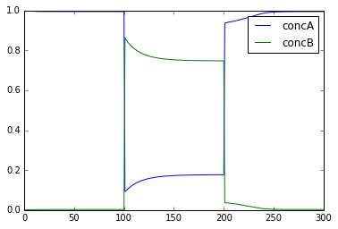
Propogation of a Bistable System
File name: propagationBis.py
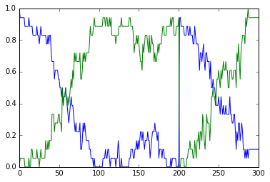
All the above models have been well-mixed, that is point or non-spatial
models. Bistables do interesting things when they are dispersed in
space. This is illustrated in this example. Here we have a tapering
cylinder, that is a pseudo 1-dimensional reaction-diffusion system.
Every point in this cylinder has the bistable system from the strongBis
example.
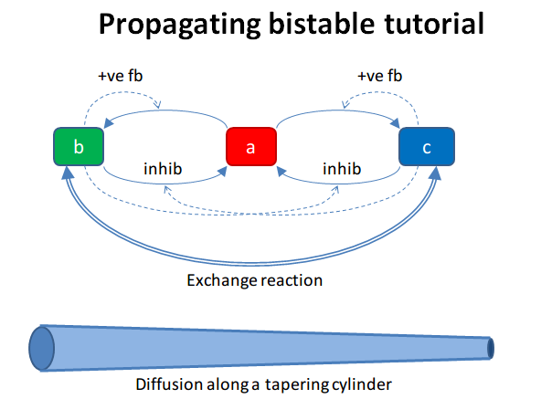
The example has two stages. First it starts out with the model in the
unstable transition point, and introduces a small symmetry-breaking
perturbation at one end. This rapidly propagates through the entire
length model, leaving molecule b at a higher value than c.
At t = 100 we carry out a different manipulation. We flip the
concentrations of molecules b and c for the left half of the model, and
then just let it run. Now we have opposing bistable states on either
half. In the middle, the two systems battle it out. Molecule c from
the left side diffuses over to the right, and tries to inhibit b,
and vice versa. However we have a small asymmetry due to the tapering of
the cylinder. As there is a slightly larger volume on the left, the
transition point gradually advances to the right, as molecule b
yields to the slightly larger amounts of molecule c.
Code:
Show/Hide code 1
2
3
4
5
6
7
8
9
10
11
12
13
14
15
16
17
18
19
20
21
22
23
24
25
26
27
28
29
30
31
32
33
34
35
36
37
38
39
40
41
42
43
44
45
46
47
48
49
50
51
52
53
54
55
56
57
58
59
60
61
62
63
64
65
66
67
68
69
70
71
72
73
74
75
76
77
78
79
80
81
82
83
84
85
86
87
88
89
90
91
92
93
94
95
96
97
98
99
100
101
102
103
104
105
106
107
108
109
110
111
112
113
114
115
116
117
118
119
120
121
122
123
124
125
126
127
128
129
130
131
132
133
134
135
136
137
138
139
140
141
142
143
144
145
146
147
148
149
150
151
152
153
154
155
156
157
158
159
160
161
162
163
164
165
166
167
168
169 | #########################################################################
## This program is part of 'MOOSE', the
## Messaging Object Oriented Simulation Environment.
## Copyright (C) 2014 Upinder S. Bhalla. and NCBS
## It is made available under the terms of the
## GNU Lesser General Public License version 2.1
## See the file COPYING.LIB for the full notice.
#########################################################################
"""
This example illustrates propagation of state flips in a
linear 1-dimensional reaction-diffusion system. It uses a
bistable system loaded in from a kkit definition file, and
places this in a tapering cylinder for pseudo 1-dimentionsional
diffusion.
This example illustrates a number of features of reaction-diffusion
calculations.
First, it shows how to set up such systems. Key steps are to create
the compartment and define its voxelization, then create the Ksolve,
Dsolve, and Stoich. Then we assign stoich.compartment, ksolve and
dsolve in that order. Finally we assign the path of the Stoich.
For running the model, we start by introducing
a small symmetry-breaking increment of concInit
of the molecule **b** in the last compartment on the cylinder. The model
starts out with molecules at equal concentrations, so that the system would
settle to the unstable fixed point. This symmetry breaking leads
to the last compartment moving towards the state with an
increased concentration of **b**,
and this effect propagates to all other compartments.
Once the model has settled to the state where **b** is high throughout,
we simply exchange the concentrations of **b** with **c** in the left
half of the cylinder. This introduces a brief transient at the junction,
which soon settles to a smooth crossover.
Finally, as we run the simulation, the tapering geometry comes into play.
Since the left hand side has a larger diameter than the right, the
state on the left gradually wins over and the transition point slowly
moves to the right.
"""
import math
import numpy
import matplotlib.pyplot as plt
import matplotlib.image as mpimg
import moose
import sys
def makeModel():
# create container for model
r0 = 1e-6 # m
r1 = 0.5e-6 # m. Note taper.
num = 200
diffLength = 1e-6 # m
comptLength = num * diffLength # m
diffConst = 20e-12 # m^2/sec
concA = 1 # millimolar
diffDt = 0.02 # for the diffusion
chemDt = 0.2 # for the reaction
mfile = '../../genesis/M1719.g'
model = moose.Neutral( 'model' )
compartment = moose.CylMesh( '/model/kinetics' )
# load in model
modelId = moose.loadModel( mfile, '/model', 'ee' )
a = moose.element( '/model/kinetics/a' )
b = moose.element( '/model/kinetics/b' )
c = moose.element( '/model/kinetics/c' )
ac = a.concInit
bc = b.concInit
cc = c.concInit
compartment.r0 = r0
compartment.r1 = r1
compartment.x0 = 0
compartment.x1 = comptLength
compartment.diffLength = diffLength
assert( compartment.numDiffCompts == num )
# Assign parameters
for x in moose.wildcardFind( '/model/kinetics/##[ISA=PoolBase]' ):
#print 'pools: ', x, x.name
x.diffConst = diffConst
# Make solvers
ksolve = moose.Ksolve( '/model/kinetics/ksolve' )
dsolve = moose.Dsolve( '/model/dsolve' )
# Set up clocks.
moose.setClock( 10, diffDt )
for i in range( 11, 17 ):
moose.setClock( i, chemDt )
stoich = moose.Stoich( '/model/kinetics/stoich' )
stoich.compartment = compartment
stoich.ksolve = ksolve
stoich.dsolve = dsolve
stoich.path = "/model/kinetics/##"
print(('dsolve.numPools, num = ', dsolve.numPools, num))
b.vec[num-1].concInit *= 1.01 # Break symmetry.
def main():
runtime = 100
displayInterval = 2
makeModel()
dsolve = moose.element( '/model/dsolve' )
moose.reinit()
#moose.start( runtime ) # Run the model for 10 seconds.
a = moose.element( '/model/kinetics/a' )
b = moose.element( '/model/kinetics/b' )
c = moose.element( '/model/kinetics/c' )
img = mpimg.imread( 'propBis.png' )
#imgplot = plt.imshow( img )
#plt.show()
plt.ion()
fig = plt.figure( figsize=(12,10) )
png = fig.add_subplot(211)
imgplot = plt.imshow( img )
ax = fig.add_subplot(212)
ax.set_ylim( 0, 0.001 )
plt.ylabel( 'Conc (mM)' )
plt.xlabel( 'Position along cylinder (microns)' )
pos = numpy.arange( 0, a.vec.conc.size, 1 )
line1, = ax.plot( pos, a.vec.conc, 'r-', label='a' )
line2, = ax.plot( pos, b.vec.conc, 'g-', label='b' )
line3, = ax.plot( pos, c.vec.conc, 'b-', label='c' )
timeLabel = plt.text(60, 0.0009, 'time = 0')
plt.legend()
fig.canvas.draw()
for t in range( displayInterval, runtime, displayInterval ):
moose.start( displayInterval )
line1.set_ydata( a.vec.conc )
line2.set_ydata( b.vec.conc )
line3.set_ydata( c.vec.conc )
timeLabel.set_text( "time = %d" % t )
fig.canvas.draw()
print('Swapping concs of b and c in half the cylinder')
for i in range( b.numData/2 ):
temp = b.vec[i].conc
b.vec[i].conc = c.vec[i].conc
c.vec[i].conc = temp
newruntime = 200
for t in range( displayInterval, newruntime, displayInterval ):
moose.start( displayInterval )
line1.set_ydata( a.vec.conc )
line2.set_ydata( b.vec.conc )
line3.set_ydata( c.vec.conc )
timeLabel.set_text( "time = %d" % (t + runtime) )
fig.canvas.draw()
print( "Hit 'enter' to exit" )
sys.stdin.read(1)
# Run the 'main' if this script is executed standalone.
if __name__ == '__main__':
main()
|
Output:

Steady-state Finder
File name: findSteadyState
This is an example of how to use an internal MOOSE solver to find steady
states of a system very rapidly. The method starts from a random
position in state space that obeys mass conservation. It then finds the
nearest steady state and reports it. If it does this enough times it
should find all the steady states.
We illustrate this process for 50 attempts to find the steady states. It
does find all of them. Each time it plots and prints the values, though
the plotting is not necessary.
The printout shows the concentrations of all molecules in the first 5
columns. Then it prints the type of solution, and the numbers of
negative and positive eigenvalues. In all cases the calculations are
successful, though it takes different numbers of iterations to arrive at
the steady state. In some models it would be necessary to put a cap on
the number of iterations, if the system is not able to find a steady
state.
In this example we run the bistable model using the ODE solver right at
the end, and manually enforce transitions to show where the target
steady states are.
For more information on the algorithm used, look in the comments within
the main method of the code below.
Code:
Show/Hide code 1
2
3
4
5
6
7
8
9
10
11
12
13
14
15
16
17
18
19
20
21
22
23
24
25
26
27
28
29
30
31
32
33
34
35
36
37
38
39
40
41
42
43
44
45
46
47
48
49
50
51
52
53
54
55
56
57
58
59
60
61
62
63
64
65
66
67
68
69
70
71
72
73
74
75
76
77
78
79
80
81
82
83
84
85
86
87
88
89
90
91
92
93
94
95
96
97
98
99
100
101
102
103
104
105
106
107
108
109
110
111
112
113
114
115
116
117
118
119
120
121
122
123
124
125
126
127
128
129
130
131
132
133
134
135
136
137
138
139
140
141
142
143
144
145
146
147
148
149
150
151
152
153
154
155
156
157
158
159
160
161
162
163
164
165
166
167
168
169
170
171
172
173
174
175
176
177
178
179
180
181
182
183
184
185
186
187
188
189
190
191
192
193 | #########################################################################
## This program is part of 'MOOSE', the
## Messaging Object Oriented Simulation Environment.
## Copyright (C) 2013 Upinder S. Bhalla. and NCBS
## It is made available under the terms of the
## GNU Lesser General Public License version 2.1
## See the file COPYING.LIB for the full notice.
#########################################################################
from __future__ import print_function
import math
import pylab
import numpy
import moose
def main():
"""
This example sets up the kinetic solver and steady-state finder, on
a bistable model of a chemical system. The model is set up within the
script.
The algorithm calls the steady-state finder 50 times with different
(randomized) initial conditions, as follows:
* Set up the random initial condition that fits the conservation laws
* Run for 2 seconds. This should not be mathematically necessary, but
for obscure numerical reasons it makes it much more likely that the
steady state solver will succeed in finding a state.
* Find the fixed point
* Print out the fixed point vector and various diagnostics.
* Run for 10 seconds. This is completely unnecessary, and is done here
just so that the resultant graph will show what kind of state has
been found.
After it does all this, the program runs for 100 more seconds on the
last found fixed point (which turns out to be a saddle node), then
is hard-switched in the script to the first attractor basin from which
it runs for another 100 seconds till it settles there, and then
is hard-switched yet again to the second attractor and runs for 400
seconds.
Looking at the output you will see many features of note:
* the first attractor (stable point) and the saddle point (unstable
fixed point) are both found quite often. But the second
attractor is found just once.
It has a very small basin of attraction.
* The values found for each of the fixed points match well with the
values found by running the system to steady-state at the end.
* There are a large number of failures to find a fixed point. These are
found and reported in the diagnostics. They show up on the plot
as cases where the 10-second runs are not flat.
If you wanted to find fixed points in a production model, you would
not need to do the 10-second runs, and you would need to eliminate the
cases where the state-finder failed. Then you could identify the good
points and keep track of how many of each were found.
There is no way to guarantee that all fixed points have been found
using this algorithm! If there are points in an obscure corner of state
space (as for the singleton second attractor convergence in this
example) you may have to iterate very many times to find them.
You may wish to sample concentration space logarithmically rather than
linearly.
"""
compartment = makeModel()
ksolve = moose.Ksolve( '/model/compartment/ksolve' )
stoich = moose.Stoich( '/model/compartment/stoich' )
stoich.compartment = compartment
stoich.ksolve = ksolve
stoich.path = "/model/compartment/##"
state = moose.SteadyState( '/model/compartment/state' )
moose.reinit()
state.stoich = stoich
state.showMatrices()
state.convergenceCriterion = 1e-6
moose.seed( 111 ) # Used when generating the samples in state space
for i in range( 0, 50 ):
getState( ksolve, state )
# Now display the states of the system at more length to compare.
moose.start( 100.0 ) # Run the model for 100 seconds.
a = moose.element( '/model/compartment/a' )
b = moose.element( '/model/compartment/b' )
# move most molecules over to b
b.conc = b.conc + a.conc * 0.9
a.conc = a.conc * 0.1
moose.start( 100.0 ) # Run the model for 100 seconds.
# move most molecules back to a
a.conc = a.conc + b.conc * 0.99
b.conc = b.conc * 0.01
moose.start( 400.0 ) # Run the model for 200 seconds.
# Iterate through all plots, dump their contents to data.plot.
displayPlots()
quit()
def makeModel():
""" This function creates a bistable reaction system using explicit
MOOSE calls rather than load from a file
"""
# create container for model
model = moose.Neutral( 'model' )
compartment = moose.CubeMesh( '/model/compartment' )
compartment.volume = 1e-15
# the mesh is created automatically by the compartment
mesh = moose.element( '/model/compartment/mesh' )
# create molecules and reactions
a = moose.Pool( '/model/compartment/a' )
b = moose.Pool( '/model/compartment/b' )
c = moose.Pool( '/model/compartment/c' )
enz1 = moose.Enz( '/model/compartment/b/enz1' )
enz2 = moose.Enz( '/model/compartment/c/enz2' )
cplx1 = moose.Pool( '/model/compartment/b/enz1/cplx' )
cplx2 = moose.Pool( '/model/compartment/c/enz2/cplx' )
reac = moose.Reac( '/model/compartment/reac' )
# connect them up for reactions
moose.connect( enz1, 'sub', a, 'reac' )
moose.connect( enz1, 'prd', b, 'reac' )
moose.connect( enz1, 'enz', b, 'reac' )
moose.connect( enz1, 'cplx', cplx1, 'reac' )
moose.connect( enz2, 'sub', b, 'reac' )
moose.connect( enz2, 'prd', a, 'reac' )
moose.connect( enz2, 'enz', c, 'reac' )
moose.connect( enz2, 'cplx', cplx2, 'reac' )
moose.connect( reac, 'sub', a, 'reac' )
moose.connect( reac, 'prd', b, 'reac' )
# Assign parameters
a.concInit = 1
b.concInit = 0
c.concInit = 0.01
enz1.kcat = 0.4
enz1.Km = 4
enz2.kcat = 0.6
enz2.Km = 0.01
reac.Kf = 0.001
reac.Kb = 0.01
# Create the output tables
graphs = moose.Neutral( '/model/graphs' )
outputA = moose.Table2 ( '/model/graphs/concA' )
outputB = moose.Table2 ( '/model/graphs/concB' )
outputC = moose.Table2 ( '/model/graphs/concC' )
outputCplx1 = moose.Table2 ( '/model/graphs/concCplx1' )
outputCplx2 = moose.Table2 ( '/model/graphs/concCplx2' )
# connect up the tables
moose.connect( outputA, 'requestOut', a, 'getConc' );
moose.connect( outputB, 'requestOut', b, 'getConc' );
moose.connect( outputC, 'requestOut', c, 'getConc' );
moose.connect( outputCplx1, 'requestOut', cplx1, 'getConc' );
moose.connect( outputCplx2, 'requestOut', cplx2, 'getConc' );
return compartment
def displayPlots():
for x in moose.wildcardFind( '/model/graphs/conc#' ):
t = numpy.arange( 0, x.vector.size, 1 ) #sec
pylab.plot( t, x.vector, label=x.name )
pylab.legend()
pylab.show()
def getState( ksolve, state ):
""" This function finds a steady state starting from a random
initial condition that is consistent with the stoichiometry rules
and the original model concentrations.
"""
scale = 1.0 / ( 1e-15 * 6.022e23 )
state.randomInit() # Randomize init conditions, subject to stoichiometry
moose.start( 2.0 ) # Run the model for 2 seconds.
state.settle() # This function finds the steady states.
for x in ksolve.nVec[0]:
print( "{:.2f}".format( x * scale ), end=' ')
print( "Type={} NegEig={} PosEig={} status={} {} Iter={:2d}".format( state.stateType, state.nNegEigenvalues, state.nPosEigenvalues, state.solutionStatus, state.status, state.nIter))
moose.start( 10.0 ) # Run model for 10 seconds, just for display
# Run the 'main' if this script is executed standalone.
if __name__ == '__main__':
main()
|
Output:
0.92 0.05 0.00 0.01 0.01 Type=2 NegEig=2 PosEig=1 status=0 success Iter=16
0.92 0.05 0.00 0.01 0.01 Type=2 NegEig=2 PosEig=1 status=0 success Iter=29
0.18 0.75 0.00 0.03 0.01 Type=0 NegEig=3 PosEig=0 status=0 success Iter=10
0.18 0.75 0.00 0.03 0.01 Type=0 NegEig=3 PosEig=0 status=0 success Iter=26
0.18 0.75 0.00 0.03 0.01 Type=0 NegEig=3 PosEig=0 status=0 success Iter=27
0.92 0.05 0.00 0.01 0.01 Type=2 NegEig=2 PosEig=1 status=0 success Iter=30
0.18 0.75 0.00 0.03 0.01 Type=0 NegEig=3 PosEig=0 status=0 success Iter=12
0.92 0.05 0.00 0.01 0.01 Type=2 NegEig=2 PosEig=1 status=0 success Iter=29
0.18 0.75 0.00 0.03 0.01 Type=0 NegEig=3 PosEig=0 status=0 success Iter=12
0.92 0.05 0.00 0.01 0.01 Type=2 NegEig=2 PosEig=1 status=0 success Iter=41
0.18 0.75 0.00 0.03 0.01 Type=0 NegEig=3 PosEig=0 status=0 success Iter=29
0.18 0.75 0.00 0.03 0.01 Type=0 NegEig=3 PosEig=0 status=0 success Iter=18
0.18 0.75 0.00 0.03 0.01 Type=0 NegEig=3 PosEig=0 status=0 success Iter=27
0.18 0.75 0.00 0.03 0.01 Type=0 NegEig=3 PosEig=0 status=0 success Iter=14
0.18 0.75 0.00 0.03 0.01 Type=0 NegEig=3 PosEig=0 status=0 success Iter=12
0.18 0.75 0.00 0.03 0.01 Type=0 NegEig=3 PosEig=0 status=0 success Iter=19
0.18 0.75 0.00 0.03 0.01 Type=0 NegEig=3 PosEig=0 status=0 success Iter= 6
0.18 0.75 0.00 0.03 0.01 Type=0 NegEig=3 PosEig=0 status=0 success Iter=14
0.18 0.75 0.00 0.03 0.01 Type=0 NegEig=3 PosEig=0 status=0 success Iter=23
0.18 0.75 0.00 0.03 0.01 Type=0 NegEig=3 PosEig=0 status=0 success Iter=25
0.18 0.75 0.00 0.03 0.01 Type=0 NegEig=3 PosEig=0 status=0 success Iter=16
0.18 0.75 0.00 0.03 0.01 Type=0 NegEig=3 PosEig=0 status=0 success Iter= 5
0.92 0.05 0.00 0.01 0.01 Type=2 NegEig=2 PosEig=1 status=0 success Iter=43
0.92 0.05 0.00 0.01 0.01 Type=2 NegEig=2 PosEig=1 status=0 success Iter= 9
0.92 0.05 0.00 0.01 0.01 Type=2 NegEig=2 PosEig=1 status=0 success Iter=43
0.92 0.05 0.00 0.01 0.01 Type=2 NegEig=2 PosEig=1 status=0 success Iter=29
0.18 0.75 0.00 0.03 0.01 Type=0 NegEig=3 PosEig=0 status=0 success Iter=27
0.18 0.75 0.00 0.03 0.01 Type=0 NegEig=3 PosEig=0 status=0 success Iter= 9
0.18 0.75 0.00 0.03 0.01 Type=0 NegEig=3 PosEig=0 status=0 success Iter=12
0.92 0.05 0.00 0.01 0.01 Type=2 NegEig=2 PosEig=1 status=0 success Iter=24
0.92 0.05 0.00 0.01 0.01 Type=2 NegEig=2 PosEig=1 status=0 success Iter=26
0.18 0.75 0.00 0.03 0.01 Type=0 NegEig=3 PosEig=0 status=0 success Iter=14
0.92 0.05 0.00 0.01 0.01 Type=2 NegEig=2 PosEig=1 status=0 success Iter=14
0.18 0.75 0.00 0.03 0.01 Type=0 NegEig=3 PosEig=0 status=0 success Iter=10
0.18 0.75 0.00 0.03 0.01 Type=0 NegEig=3 PosEig=0 status=0 success Iter=13
0.18 0.75 0.00 0.03 0.01 Type=0 NegEig=3 PosEig=0 status=0 success Iter=26
0.18 0.75 0.00 0.03 0.01 Type=0 NegEig=3 PosEig=0 status=0 success Iter=21
0.18 0.75 0.00 0.03 0.01 Type=0 NegEig=3 PosEig=0 status=0 success Iter=26
0.18 0.75 0.00 0.03 0.01 Type=0 NegEig=3 PosEig=0 status=0 success Iter=24
0.18 0.75 0.00 0.03 0.01 Type=0 NegEig=3 PosEig=0 status=0 success Iter=24
0.92 0.05 0.00 0.01 0.01 Type=2 NegEig=2 PosEig=1 status=0 success Iter=18
0.18 0.75 0.00 0.03 0.01 Type=0 NegEig=3 PosEig=0 status=0 success Iter=26
0.18 0.75 0.00 0.03 0.01 Type=5 NegEig=4 PosEig=0 status=0 success Iter=13
0.18 0.75 0.00 0.03 0.01 Type=0 NegEig=3 PosEig=0 status=0 success Iter=23
0.92 0.05 0.00 0.01 0.01 Type=2 NegEig=2 PosEig=1 status=0 success Iter=24
0.18 0.75 0.00 0.03 0.01 Type=0 NegEig=3 PosEig=0 status=0 success Iter= 8
0.18 0.75 0.00 0.03 0.01 Type=0 NegEig=3 PosEig=0 status=0 success Iter=18
0.18 0.75 0.00 0.03 0.01 Type=0 NegEig=3 PosEig=1 status=0 success Iter=21
0.99 0.00 0.01 0.00 0.00 Type=0 NegEig=3 PosEig=0 status=0 success Iter=15
0.92 0.05 0.00 0.01 0.01 Type=2 NegEig=2 PosEig=1 status=0 success Iter=29
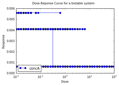
Dose Response (Under construction)
File name: doseResponse.py
This example generates a doseResponse plot for a bistable system,
against a control parameter (dose) that takes the system in and out
again from the bistable regime. Like the previous example, it uses the
steady-state solver to find the stable points for each value of the
control parameter. Unfortunately it doesn't work right now. Seems like
the kcat scaling isn't being registered.
Code:
Show/Hide code 1
2
3
4
5
6
7
8
9
10
11
12
13
14
15
16
17
18
19
20
21
22
23
24
25
26
27
28
29
30
31
32
33
34
35
36
37
38
39
40
41
42
43
44
45
46
47
48
49
50
51
52
53
54
55
56
57
58
59
60
61
62
63
64
65
66
67
68
69
70
71
72
73
74
75
76
77
78
79
80
81
82
83
84
85
86
87
88
89
90
91
92
93
94
95
96
97
98
99
100
101
102
103
104
105
106
107
108
109
110
111
112
113
114
115
116
117
118
119
120
121
122
123
124
125 | ## Makes and plots the dose response curve for bistable models
## Author: Sahil Moza
## June 26, 2014
import moose
import pylab
import numpy as np
from matplotlib import pyplot as plt
def setupSteadyState(simdt,plotDt):
ksolve = moose.Ksolve( '/model/kinetics/ksolve' )
stoich = moose.Stoich( '/model/kinetics/stoich' )
stoich.compartment = moose.element('/model/kinetics')
stoich.ksolve = ksolve
#ksolve.stoich = stoich
stoich.path = "/model/kinetics/##"
state = moose.SteadyState( '/model/kinetics/state' )
#### Set clocks here
#moose.useClock(4, "/model/kinetics/##[]", "process")
#moose.setClock(4, float(simdt))
#moose.setClock(5, float(simdt))
#moose.useClock(5, '/model/kinetics/ksolve', 'process' )
#moose.useClock(8, '/model/graphs/#', 'process' )
#moose.setClock(8, float(plotDt))
moose.reinit()
state.stoich = stoich
state.showMatrices()
state.convergenceCriterion = 1e-8
return ksolve, state
def parseModelName(fileName):
pos1=fileName.rfind('/')
pos2=fileName.rfind('.')
directory=fileName[:pos1]
prefix=fileName[pos1+1:pos2]
suffix=fileName[pos2+1:len(fileName)]
return directory, prefix, suffix
# Solve for the steady state
def getState( ksolve, state, vol):
scale = 1.0 / ( vol * 6.022e23 )
moose.reinit
state.randomInit() # Removing random initial condition to systematically make Dose reponse curves.
moose.start( 2.0 ) # Run the model for 2 seconds.
state.settle()
vector = []
a = moose.element( '/model/kinetics/a' ).conc
for x in ksolve.nVec[0]:
vector.append( x * scale)
moose.start( 10.0 ) # Run model for 10 seconds, just for display
failedSteadyState = any([np.isnan(x) for x in vector])
if not (failedSteadyState):
return state.stateType, state.solutionStatus, a, vector
def main():
# Setup parameters for simulation and plotting
simdt= 1e-2
plotDt= 1
# Factors to change in the dose concentration in log scale
factorExponent = 10 ## Base: ten raised to some power.
factorBegin = -20
factorEnd = 21
factorStepsize = 1
factorScale = 10.0 ## To scale up or down the factors
# Load Model and set up the steady state solver.
# model = sys.argv[1] # To load model from a file.
model = './19085.cspace'
modelPath, modelName, modelType = parseModelName(model)
outputDir = modelPath
modelId = moose.loadModel(model, 'model', 'ee')
dosePath = '/model/kinetics/b/DabX' # The dose entity
ksolve, state = setupSteadyState( simdt, plotDt)
vol = moose.element( '/model/kinetics' ).volume
iterInit = 100
solutionVector = []
factorArr = []
enz = moose.element(dosePath)
init = enz.kcat # Dose parameter
# Change Dose here to .
for factor in range(factorBegin, factorEnd, factorStepsize ):
scale = factorExponent ** (factor/factorScale)
enz.kcat = init * scale
print( "scale={:.3f}\tkcat={:.3f}".format( scale, enz.kcat) )
for num in range(iterInit):
stateType, solStatus, a, vector = getState( ksolve, state, vol)
if solStatus == 0:
#solutionVector.append(vector[0]/sum(vector))
solutionVector.append(a)
factorArr.append(scale)
joint = np.array([factorArr, solutionVector])
joint = joint[:,joint[1,:].argsort()]
# Plot dose response.
fig0 = plt.figure()
pylab.semilogx(joint[0,:],joint[1,:],marker="o",label = 'concA')
pylab.xlabel('Dose')
pylab.ylabel('Response')
pylab.suptitle('Dose-Reponse Curve for a bistable system')
pylab.legend(loc=3)
#plt.savefig(outputDir + "/" + modelName +"_doseResponse" + ".png")
plt.show()
#plt.close(fig0)
quit()
if __name__ == '__main__':
main()
|
Output:
scale=0.010 kcat=0.004
scale=0.013 kcat=0.005
scale=0.016 kcat=0.006
scale=0.020 kcat=0.007
scale=0.025 kcat=0.009
scale=0.032 kcat=0.011
scale=0.040 kcat=0.014
scale=0.050 kcat=0.018
scale=0.063 kcat=0.023
scale=0.079 kcat=0.029
scale=0.100 kcat=0.036
scale=0.126 kcat=0.045
scale=0.158 kcat=0.057
scale=0.200 kcat=0.072
scale=0.251 kcat=0.091
scale=0.316 kcat=0.114
scale=0.398 kcat=0.144
scale=0.501 kcat=0.181
scale=0.631 kcat=0.228
scale=0.794 kcat=0.287
scale=1.000 kcat=0.361
scale=1.259 kcat=0.454
scale=1.585 kcat=0.572
scale=1.995 kcat=0.720
scale=2.512 kcat=0.907
scale=3.162 kcat=1.142
scale=3.981 kcat=1.437
scale=5.012 kcat=1.809
scale=6.310 kcat=2.278
scale=7.943 kcat=2.868
scale=10.000        kcat=3.610
scale=12.589        kcat=4.545
scale=15.849        kcat=5.722
scale=19.953        kcat=7.203
scale=25.119        kcat=9.068
scale=31.623        kcat=11.416
scale=39.811        kcat=14.372
scale=50.119        kcat=18.093
scale=63.096        kcat=22.778
scale=79.433        kcat=28.676
scale=100.000       kcat=36.101