Chemical Oscillators¶

Chemical Oscillators, also known as chemical clocks, are chemical systems in which the concentrations of one or more reactants undergoes periodic changes.

These Oscillatory reactions can be modelled using moose. The examples below demonstrate different types of chemical oscillators, as well as how they can be simulated using moose. Each example has a short description, the code used in the simulation, and the default (gsl solver) output of the code.

Each example can be found as a python file within the main moose folder under

(...)/moose/moose-examples/tutorials/ChemicalOscillators

In order to run the example, run the script

python filename.py

in command line, where filename.py is the name of the python file you would like to run. The filenames of each example are written in bold at the beginning of their respective sections, and the files themselves can be found in the aformentioned directory.

In chemical models that use solvers, there are optional arguments that allow you to specify which solver you would like to use.

python filename.py [gsl | gssa | ee]

Where:

gsl: This is the Runge-Kutta-Fehlberg implementation from the GNU Scientific Library (GSL). It is a fifth order variable timestep explicit method. Works well for most reaction systems except if they have very stiff reactions.

gssl: Optimized Gillespie stochastic systems algorithm, custom implementation. This uses variable timesteps internally. Note that it slows down with increasing numbers of molecules in each pool. It also slows down, but not so badly, if the number of reactions goes up.

Exponential Euler:This methods computes the solution of partial and ordinary differential equations.

All the following examples can be run with either of the three solvers, each of which has different advantages and disadvantages and each of which might produce a slightly different outcome.

Simply running the file without the optional argument will by default use the gsl solver. These gsl outputs are the ones shown below.

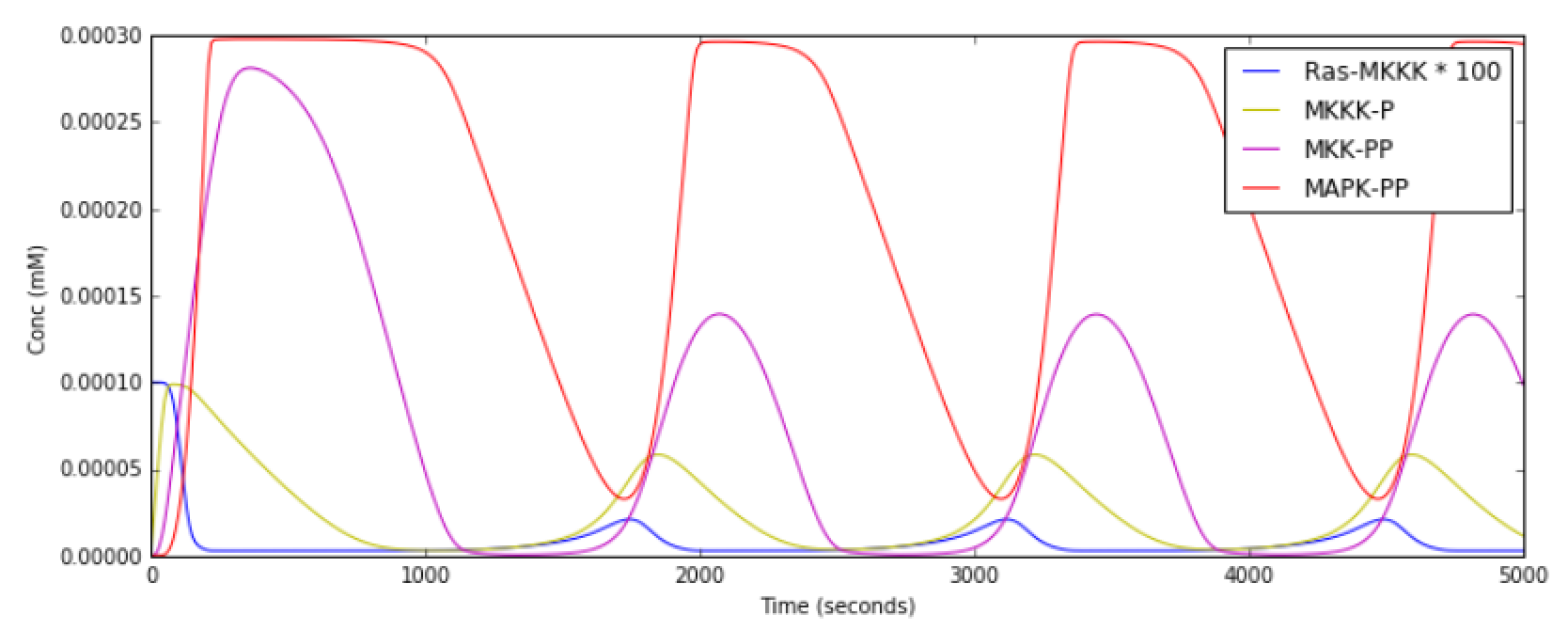
Slow Feedback Oscillator¶

File name: slowFbOsc.py

This example illustrates loading, and running a kinetic model for a delayed -ve feedback oscillator, defined in kkit format. The model is one by Boris N. Kholodenko from Eur J Biochem. (2000) 267(6):1583-8

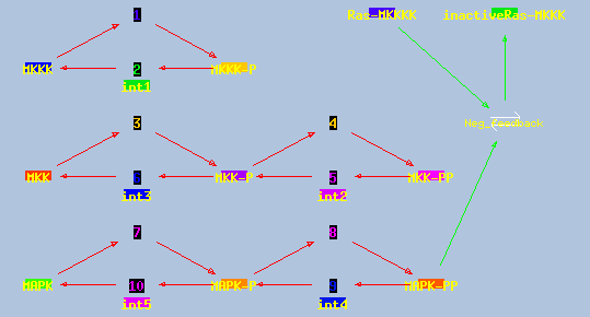
This model has a high-gain MAPK stage, whose effects are visible whem one looks at the traces from successive stages in the plots. The upstream pools have small early peaks, and the downstream pools have large delayed ones. The negative feedback step is mediated by a simple binding reaction of the end-product of oscillation with an upstream activator.

We use the gsl solver here. The model already defines some plots and sets the runtime to 4000 seconds. The model does not really play nicely with the GSSA solver, since it involves some really tiny amounts of the MAPKKK.

Things to do with the model:

- Look at model once it is loaded in::

        moose.le( '/model' )
        moose.showfields( '/model/kinetics/MAPK/MAPK' )

- Behold the amplification properties of the cascade. Could do this by blocking the feedback step and giving a small pulse input.
- Suggest which parameters you would alter to change the period of the oscillator:
    - Concs of various molecules, for example::

        ras_MAPKKKK = moose.element( '/model/kinetics/MAPK/Ras_dash_MKKKK' )
        moose.showfields( ras_MAPKKKK )
        ras_MAPKKKK.concInit = 1e-5
    - Feedback reaction rates
    - Rates of all the enzymes::

        for i in moose.wildcardFind( '/##[ISA=EnzBase]'):
                i.kcat *= 10.0

Code:

Show/Hide code

Output:

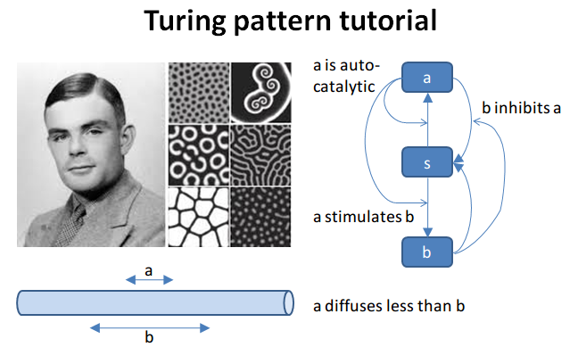
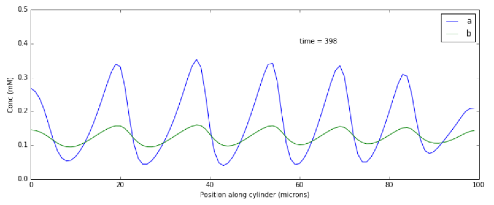
Turing Pattern Oscillator in One Dimension¶

File name: TuringOneDim.py

This example illustrates how to set up a oscillatory Turing pattern in 1-D using reaction diffusion calculations. Reaction system is:

s ---a---> a  // s goes to a, catalyzed by a.
s ---a---> b  // s goes to b, catalyzed by a.
a ---b---> s  // a goes to s, catalyzed by b.
b -------> s  // b is degraded irreversibly to s.

in sum, a has a positive feedback onto itself and also forms b. b has a negative feedback onto a. Finally, the diffusion constant for a is 1/10 that of b.

This chemical system is present in a 1-dimensional (cylindrical) compartment. The entire reaction-diffusion system is set up within the script.

Code:

Show/Hide code

#########################################################################
## This program is part of 'MOOSE', the
## Messaging Object Oriented Simulation Environment.
##           Copyright (C) 2014 Upinder S. Bhalla. and NCBS
## It is made available under the terms of the
## GNU Lesser General Public License version 2.1
## See the file COPYING.LIB for the full notice.
#########################################################################

import math
import numpy
import matplotlib.pyplot as plt
import matplotlib.image as mpimg
import moose

def makeModel():

    # create container for model
    r0 = 1e-6       # m
    r1 = 1e-6       # m
    num = 100
    diffLength = 1e-6 # m
    len = num * diffLength  # m
    diffConst = 5e-12 # m^2/sec
    motorRate = 1e-6 # m/sec
    concA = 1 # millimolar
    dt4 = 0.02  # for the diffusion
    dt5 = 0.2   # for the reaction

    model = moose.Neutral( 'model' )
    compartment = moose.CylMesh( '/model/compartment' )
    compartment.r0 = r0
    compartment.r1 = r1
    compartment.x0 = 0
    compartment.x1 = len
    compartment.diffLength = diffLength

    assert( compartment.numDiffCompts == num )

    # create molecules and reactions
    a = moose.Pool( '/model/compartment/a' )
    b = moose.Pool( '/model/compartment/b' )
    s = moose.Pool( '/model/compartment/s' )
    e1 = moose.MMenz( '/model/compartment/e1' )
    e2 = moose.MMenz( '/model/compartment/e2' )
    e3 = moose.MMenz( '/model/compartment/e3' )
    r1 = moose.Reac( '/model/compartment/r1' )
    moose.connect( e1, 'sub', s, 'reac' )
    moose.connect( e1, 'prd', a, 'reac' )
    moose.connect( a, 'nOut', e1, 'enzDest' )
    e1.Km = 1
    e1.kcat = 1

    moose.connect( e2, 'sub', s, 'reac' )
    moose.connect( e2, 'prd', b, 'reac' )
    moose.connect( a, 'nOut', e2, 'enzDest' )
    e2.Km = 1
    e2.kcat = 0.5

    moose.connect( e3, 'sub', a, 'reac' )
    moose.connect( e3, 'prd', s, 'reac' )
    moose.connect( b, 'nOut', e3, 'enzDest' )
    e3.Km = 0.1
    e3.kcat = 1

    moose.connect( r1, 'sub', b, 'reac' )
    moose.connect( r1, 'prd', s, 'reac' )
    r1.Kf = 0.3 # 1/sec
    r1.Kb = 0 # 1/sec

    # Assign parameters
    a.diffConst = diffConst/10
    b.diffConst = diffConst
    s.diffConst = 0

    # Make solvers
    ksolve = moose.Ksolve( '/model/compartment/ksolve' )
    dsolve = moose.Dsolve( '/model/dsolve' )
    # Set up clocks. The dsolver to know before assigning stoich
    moose.setClock( 4, dt4 )
    moose.setClock( 5, dt5 )
    moose.useClock( 4, '/model/dsolve', 'process' )
    # Ksolve must be scheduled after dsolve.
    moose.useClock( 5, '/model/compartment/ksolve', 'process' )

    stoich = moose.Stoich( '/model/compartment/stoich' )
    stoich.compartment = compartment
    stoich.ksolve = ksolve
    stoich.dsolve = dsolve
    stoich.path = "/model/compartment/##"
    assert( dsolve.numPools == 3 )
    a.vec.concInit = [0.1]*num
    a.vec[0].concInit *= 1.2 # slight perturbation at one end.
    b.vec.concInit = [0.1]*num
    s.vec.concInit = [1]*num

def displayPlots():
    a = moose.element( '/model/compartment/a' )
    b = moose.element( '/model/compartment/b' )
    pos = numpy.arange( 0, a.vec.conc.size, 1 )
    pylab.plot( pos, a.vec.conc, label='a' )
    pylab.plot( pos, b.vec.conc, label='b' )
    pylab.legend()
    pylab.show()

def main():
    runtime = 400
    displayInterval = 2
    makeModel()
    dsolve = moose.element( '/model/dsolve' )
    moose.reinit()
    #moose.start( runtime ) # Run the model for 10 seconds.

    a = moose.element( '/model/compartment/a' )
    b = moose.element( '/model/compartment/b' )
    s = moose.element( '/model/compartment/s' )

    img = mpimg.imread( 'turingPatternTut.png' )
    #imgplot = plt.imshow( img )
    #plt.show()

    plt.ion()
    fig = plt.figure( figsize=(12,10) )
    png = fig.add_subplot(211)
    imgplot = plt.imshow( img )
    ax = fig.add_subplot(212)
    ax.set_ylim( 0, 0.5 )
    plt.ylabel( 'Conc (mM)' )
    plt.xlabel( 'Position along cylinder (microns)' )
    pos = numpy.arange( 0, a.vec.conc.size, 1 )
    line1, = ax.plot( pos, a.vec.conc, label='a' )
    line2, = ax.plot( pos, b.vec.conc, label='b' )
    timeLabel = plt.text(60, 0.4, 'time = 0')
    plt.legend()
    fig.canvas.draw()

    for t in range( displayInterval, runtime, displayInterval ):
        moose.start( displayInterval )
        line1.set_ydata( a.vec.conc )
        line2.set_ydata( b.vec.conc )
        timeLabel.set_text( "time = %d" % t )
        fig.canvas.draw()

    print( "Hit 'enter' to exit" )
    raw_input( )



# Run the 'main' if this script is executed standalone.
if __name__ == '__main__':
    main()

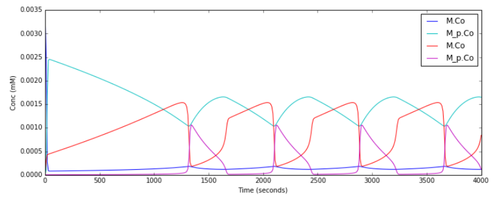
Output:

Relaxation Oscillator¶

File name: relaxationOsc.py

This example illustrates a Relaxation Oscillator. This is an oscillator built around a switching reaction, which tends to flip into one or other state and stay there. The relaxation bit comes in because once it is in state 1, a slow (relaxation) process begins which eventually flips it into state 2, and vice versa.

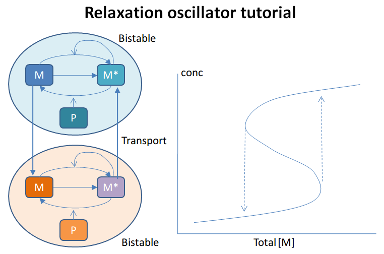
The model is based on Bhalla, Biophys J. 2011. It is defined in kkit format. It uses the deterministic gsl solver by default. You can specify the stochastic Gillespie solver on the command line

``python relaxationOsc.py gssa``

Things to do with the model:

* Figure out what determines its frequency. You could change
  the initial concentrations of various model entities::

    ma = moose.element( '/model/kinetics/A/M' )
    ma.concInit *= 1.5

  Alternatively, you could scale the rates of molecular traffic
  between the compartments::

    exo = moose.element( '/model/kinetics/exo' )
    endo = moose.element( '/model/kinetics/endo' )
    exo.Kf *= 1.0
    endo.Kf *= 1.0

* Play with stochasticity. The standard thing here is to scale the
  volume up and down::

    compt.volume = 1e-18
    compt.volume = 1e-20
    compt.volume = 1e-21

Code:

Show/Hide code

#########################################################################
## This program is part of 'MOOSE', the
## Messaging Object Oriented Simulation Environment.
##           Copyright (C) 2014 Upinder S. Bhalla. and NCBS
## It is made available under the terms of the
## GNU Lesser General Public License version 2.1
## See the file COPYING.LIB for the full notice.
#########################################################################

import moose
import matplotlib.pyplot as plt
import matplotlib.image as mpimg
import pylab
import numpy
import sys

def main():

    solver = "gsl"  # Pick any of gsl, gssa, ee..
    #solver = "gssa"  # Pick any of gsl, gssa, ee..
    mfile = '../../genesis/OSC_Cspace.g'
    runtime = 4000.0
    if ( len( sys.argv ) >= 2 ):
            solver = sys.argv[1]
    modelId = moose.loadModel( mfile, 'model', solver )
    # Increase volume so that the stochastic solver gssa
    # gives an interesting output
    compt = moose.element( '/model/kinetics' )
    compt.volume = 1e-19
    dt = moose.element( '/clock' ).tickDt[18] # 18 is the plot clock.

    moose.reinit()
    moose.start( runtime )

    # Display all plots.
    img = mpimg.imread( 'relaxOsc_tut.png' )
    fig = plt.figure( figsize=(12, 10 ) )
    png = fig.add_subplot( 211 )
    imgplot = plt.imshow( img )
    ax = fig.add_subplot( 212 )
    x = moose.wildcardFind( '/model/#graphs/conc#/#' )
    t = numpy.arange( 0, x[0].vector.size, 1 ) * dt
    ax.plot( t, x[0].vector, 'b-', label=x[0].name )
    ax.plot( t, x[1].vector, 'c-', label=x[1].name )
    ax.plot( t, x[2].vector, 'r-', label=x[2].name )
    ax.plot( t, x[3].vector, 'm-', label=x[3].name )
    plt.ylabel( 'Conc (mM)' )
    plt.xlabel( 'Time (seconds)' )
    pylab.legend()
    pylab.show()

# Run the 'main' if this script is executed standalone.
if __name__ == '__main__':
    main()

Output:

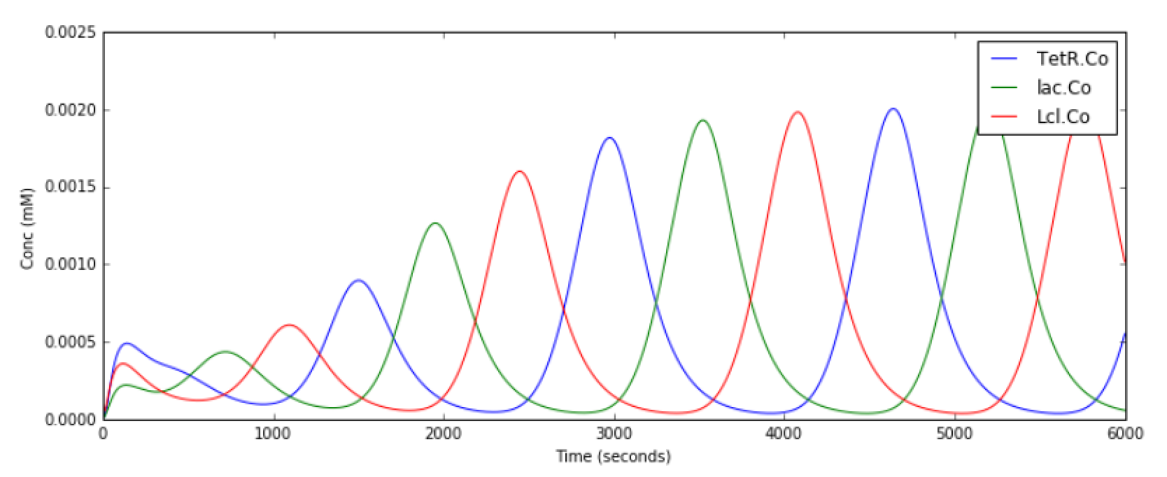
Repressilator¶

File name: repressilator.py

This example illustrates the classic Repressilator model, based on Elowitz and Liebler, Nature 2000. The model has the basic architecture

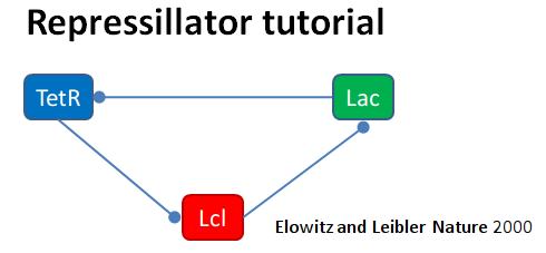
where TetR, Lac, and Lcl are genes whose products repress eachother. The circle symbol indicates inhibition. The model uses the Gillespie (stochastic) method by default but you can run it using a deterministic method by saying python repressillator.py gsl

Good things to do with this model include:

* Ask what it would take to change period of repressillator:

    * Change inhibitor rates::

        inhib = moose.element( '/model/kinetics/TetR_gene/inhib_reac' )
        moose.showfields( inhib )
        inhib.Kf *= 0.1

    * Change degradation rates::

        degrade = moose.element( '/model/kinetics/TetR_gene/TetR_degradation' )
        degrade.Kf *= 10.0
* Run in stochastic mode:

    * Change volumes, figure out how many molecules are present::

        lac = moose.element( '/model/kinetics/lac_gene/lac' )
        print lac.n``

    * Find when it becomes hopelessly unreliable with small volumes.

Code:

Show/Hide code

Output: