Simple Examples

How to run these examples

Each of the following examples can be run by clicking on the green source button
on the right side of each example, and running from within a ``.py`` python file
on a computer where moose is installed.

Alternatively, all the files mentioned on this page can be found in the main
moose directory. They can be found under

    (...)/moose/moose-examples/snippets

They can be run by typing

    $ python filename.py

in your command line, where filename.py is the python file you want to run.

All of the following examples show one or more methods within each python file.
For example, in the ``cubeMeshSigNeur`` section, there are two blue tabs
describing the ``cubeMeshSigNeur.createSquid()`` and ``cubeMeshSigNeur.main()``
methods.

The filename is the bit that comes before the ``.`` in the blue boxes, with
``.py`` added at the end of it. In this case, the file name would be
``cubeMeshSigNeur.py``.

Set-up a kinetic solver and model

with Scripting

scriptGssaSolver.main()

This example illustrates how to set up a kinetic solver and kinetic model using the scripting interface. Normally this would be done using the Shell::doLoadModel command, and normally would be coordinated by the SimManager as the base of the entire model. This example creates a bistable model having two enzymes and a reaction. One of the enzymes is autocatalytic. The model is set up to run using Exponential Euler integration.

With something else

changeFuncExpression.main()

This example illustrates how to set up a kinetic solver and kinetic model using the scripting interface. Normally this would be done using the Shell::doLoadModel command, and normally would be coordinated by the SimManager as the base of the entire model. This example creates a bistable model having two enzymes and a reaction. One of the enzymes is autocatalytic. The model is set up to run using Exponential Euler integration.

Building a chemical Model from Parts

Disclaimer: Avoid doing this for all but the very simplest models. This is error-prone, tedious, and non-portable. For preference use one of the standard model formats like SBML, which MOOSE and many other tools can read and write.

Nevertheless, it is useful to see how these models are set up. There are several tutorials and snippets that build the entire chemical model system using the basic MOOSE calls. The sequence of steps is typically:

1. Create container (chemical compartment) for model. This is typically a CubeMesh, a CylMesh, and if you really know what you are doing, a NeuroMesh.

2. Create the reaction components: pools of molecules moose.Pool; reactions moose.Reac; and enzymes moose.Enz. Note that when creating an enzyme, one must also create a molecule beneath it to serve as the enzyme-substrate complex. Other less-used components include Michaelis-Menten enzymes moose.MMenz, input tables, pulse generators and so on. These are illustrated in other examples. All these reaction components should be child objects of the compartment, since this defines what volume they will occupy. Specifically , a pool or reaction object must be placed somewhere below the compartment in the object tree for the volume to be set correctly and for the solvers to know what to use.

3. Assign parameters for the components.

   • Compartments have a volume, and each subtype will have quite elaborate options for partitioning the compartment into voxels.
   • Pool s have one key parameter, the initial concentration concInit.
   • Reac tions have two parameters: K_f and K_b.
   • Enz ymes have two primary parameters k_cat and K_m. That is enough for MMenz ymes. Regular Enz ymes have an additional parameter k₂ which by default is set to 4.0 times k_cat, but you may also wish to explicitly assign it if you know its value.

4. Connect up the reaction system using moose messaging.

5. Create and connect up input and output tables as needed.

6. Create and connect up the solvers as needed. This has to be done in a specific order. Examples are linked below, but briefly the order is:

   1. Make the compartment and reaction system.
   2. Make the Ksolve or Gsolve.
   3. Make the Stoich.
   4. Assign stoich.compartment to the compartment
   5. Assign stoich.ksolve to either the Ksolve or Gsolve.
   6. Assign stoich.path to finally fill in the reaction system.

An example of manipulating the models is as following:

scriptKineticSolver.main()

This example illustrates how to set up a kinetic solver and kinetic model using the scripting interface. Normally this would be done using the Shell::doLoadModel command, and normally would be coordinated by the SimManager as the base of the entire model. This example creates a bistable model having two enzymes and a reaction. One of the enzymes is autocatalytic. The model is set up to run using Exponential Euler integration.

The recommended way to build a chemical model, of course, is to load it in from a file format specific to such models. MOOSE understands SBML, kkit.g (a legacy GENESIS format), and cspace (a very compact format used in a large study of bistables from Ramakrishnan and Bhalla, PLoS Comp. Biol 2008).

One key concept is that in MOOSE the components, messaging, and access to model components is identical regardless of whether the model was built from parts, or loaded in from a file. All that the file loaders do is to use the file to automate the steps above. Thus the model components and their fields are completely accessible from the script even if the model has been loaded from a file.

Cross-Compartment Reaction Systems

Frequently reaction systems span cellular (chemical) compartments. For example, a membrane-bound molecule may be phosphorylated by a cytosolic kinase, using soluble ATP as one of the substrates. Here the membrane and the cytsol are different chemical compartments. MOOSE supports such reactions. The following snippets illustrate cross-compartment chemistry. Note that the interpretation of the rates of enzymes and reactions does depend on which compartment they reside in.

crossComptSimpleReac.main()

This example illustrates a simple cross compartment reaction:

a <===> b <===> c

Here each molecule is in a different compartment. The initial conditions are such that the end concentrations on all compartments should be 2.0. The time course depends on which compartment the Reac object is embedded in. The cleanest thing numerically and also conceptually is to have both reactions in the same compartment, in this case the middle one (compt1). The initial conditions have a lot of B. The equilibrium with C is fast and so C shoots up and passes B, peaking at about (2.5,9). This is also just about the crossover point. A starts low and slowly climbs up to equilibrate.

If we put reac0 in compt0 and reac1 in compt1, it behaves the same qualitiatively but now the peak is at around (1, 5.2)

This configuration of reactions makes sense from the viewpoint of having the reactions always in the compartment with the smaller volume, which is important if we need to have junctions where many small voxels talk to one big voxel in another compartment.

Note that putting the reacs in other compartments doesn't work and in some combinations (e.g., reac0 in compt0 and reac1 in compt2) give numerical instability.

crossComptNeuroMesh.main()

This example illustrates how to define a kinetic model embedded in a NeuroMesh, and undergoing cross-compartment reactions. It is completely self-contained and does not use any external model definition files. Normally one uses standard model formats like SBML or kkit to concisely define kinetic and neuronal models. This example creates a simple reaction:

a <==> b <==> c

in which a, b, and c are in the dendrite, spine head, and PSD respectively. The model is set up to run using the Ksolve for integration. Although a diffusion solver is set up, the diff consts here are set to zero. The display has two parts: Above is a line plot of concentration against compartment#. Below is a time-series plot that appears after # the simulation has ended. The plot is for the last (rightmost) compartment. Concentrations of a, b, c are plotted for both graphs.

crossComptSimpleReacGSSA.main()

This example illustrates a simple cross compartment reaction:

a <===> b <===> c

Here each molecule is in a different compartment. The initial conditions are such that the end conc on all compartments should be 2.0. The time course depends on which compartment the Reac object is embedded in. The cleanest thing numerically and also conceptually is to have both reactions in the same compartment, in this case the middle one (compt1). The initial conditions have a lot of B. The equilibrium with C is fast and so C shoots up and passes B, peaking at about (2.5,9). This is also just about the crossover point. A starts low and slowly climbs up to equilibrate.

If we put reac0 in compt0 and reac1 in compt1, it behaves the same qualitiatively but now the peak is at around (1, 5.2)

This configuration of reactions makes sense from the viewpoint of having the reactions always in the compartment with the smaller volume, which is important if we need to have junctions where many small voxels talk to one big voxel in another compartment.

Note that putting the reacs in other compartments doesn't work and in some combinations (e.g., reac0 in compt0 and reac1 in compt2) give numerical instability.

Tweaking Parameters

tweakingParameters.main()

This example illustrates parameter tweaking. It uses a kinetic model for a relaxation oscillator, defined in kkit format. We use the gsl solver here. The model looks like this:

        _________
        |        |
        V        |
M-----Enzyme---->M*           All in compartment A
|\             /| ^
| \___basal___/   |
|                 |
endo              |
|                 exo
|       _______   |
|       |      \  |
V       V       \ |
M-----Enzyme---->M*           All in compartment B
\             /|
\___basal___/

The way it works: We set the run off for a few seconds with the original model parameters. This version oscillates. Then we double the endo and exo forward rates and run it further to show that the period becomes nearly twice as fast. Then we restore endo and exo, and instead double the initial amounts of M. We run it further again to see what happens.

Models' Demonstration

Oscillation Model

repressillator.main()

This example illustrates the classic Repressilator model, based on Elowitz and Liebler, Nature 2000. The model has the basic architecture:

A ---| B---| C
T            |
|            |
|____________|

where A, B, and C are genes whose products repress eachother. The plunger symbol indicates inhibition. The model uses the Gillespie (stochastic) method by default but you can run it using a deterministic method by saying python repressillator.py gsl

Good things to do with this model include:

• Ask what it would take to change period of repressillator:

  • Change inhibitor rates:

    inhib = moose.element( '/model/kinetics/TetR_gene/inhib_reac' )
    moose.showfields( inhib )
    inhib.Kf *= 0.1
    

  • Change degradation rates:

    degrade = moose.element( '/model/kinetics/TetR_gene/TetR_degradation' )
    degrade.Kf *= 10.0
    

• Run in stochastic mode:

  • Change volumes, figure out how many molecules are present:

    lac = moose.element( '/model/kinetics/lac_gene/lac' )
    print lac.n``
    

  • Find when it becomes hopelessly unreliable with small volumes.

relaxationOsc.main()

This example illustrates a Relaxation Oscillator. This is an oscillator built around a switching reaction, which tends to flip into one or other state and stay there. The relaxation bit comes in because once it is in state 1, a slow (relaxation) process begins which eventually flips it into state 2, and vice versa.

The model is based on Bhalla, Biophys J. 2011. It is defined in kkit format. It uses the deterministic gsl solver by default. You can specify the stochastic Gillespie solver on the command line python relaxationOsc.py gssa

Things to do with the model:

• Figure out what determines its frequency. You could change the initial concentrations of various model entities:

  ma = moose.element( '/model/kinetics/A/M' )
  ma.concInit *= 1.5
  

  Alternatively, you could scale the rates of molecular traffic between the compartments:

  exo = moose.element( '/model/kinetics/exo' )
  endo = moose.element( '/model/kinetics/endo' )
  exo.Kf *= 1.0
  endo.Kf *= 1.0
  

• Play with stochasticity. The standard thing here is to scale the volume up and down:

  compt.volume = 1e-18 
  compt.volume = 1e-20 
  compt.volume = 1e-21 
  

Bistability Models

MAPK feedback loop model

mapkFB.main()

This example illustrates loading, and running a kinetic model for a bistable positive feedback system, defined in kkit format. This is based on Bhalla, Ram and Iyengar, Science 2002.

The core of this model is a positive feedback loop comprising of the MAPK cascade, PLA2, and PKC. It receives PDGF and Ca2+ as inputs.

This model is quite a large one and due to some stiffness in its equations, it runs somewhat slowly.

The simulation illustrated here shows how the model starts out in a state of low activity. It is induced to 'turn on' when a a PDGF stimulus is given for 400 seconds. After it has settled to the new 'on' state, model is made to 'turn off' by setting the system calcium levels to zero for a while. This is a somewhat unphysiological manipulation!

Simple minimal bistable model

scaleVolumes.main()

This example illustrates how to run a model at different volumes. The key line is just to set the volume of the compartment:

compt.volume = vol

If everything else is set up correctly, then this change propagates through to all reactions molecules.

For a deterministic reaction one would not see any change in output concentrations. For a stochastic reaction illustrated here, one sees the level of 'noise' changing, even though the concentrations are similar up to a point. This example creates a bistable model having two enzymes and a reaction. One of the enzymes is autocatalytic. This model is set up within the script rather than using an external file. The model is set up to run using the GSSA (Gillespie Stocahstic systems algorithim) method in MOOSE.

To run the example, run the script

python scaleVolumes.py

and hit enter every cycle to see the outcome of stochastic calculations at ever smaller volumes, keeping concentrations the same.

Strongly bistable Model

strongBis.main()

This example illustrates loading, and running a kinetic model for a bistable system, defined in kkit format. Defaults to the deterministic gsl method, you can pick the stochastic one by

python filename gssa

The model starts out equally poised between sides b and c. Then there is a small molecular 'tap' to push it over to b. Then we apply a moderate push to show that it is now very stably in this state. it takes a strong push to take it over to c. Then it takes a strong push to take it back to b. This is a good model to use as the basis for running stochastically and examining how state stability is affected by changing volume.

Model of bidirectional synaptic plasticity

[showing bistable chemical switch]

bidirectionalPlasticity.main()

This is a toy model of synaptic bidirectional plasticity. The model has a small bistable chemical switch, and a small set of reactions that decode calcium input. One can turn the switch on with short high calcium pulses (over 2 uM for about 10 sec). One can turn it back off again using a long, lower calcium pulse (0.2 uM, 2000 sec).

Reaction Diffusion Models

The MOOSE design for reaction-diffusion is to specify one or more cellular 'compartments', and embed reaction systems in each of them.

A 'compartment', in the context of reaction-diffusion, is used in the cellular sense of a biochemically defined, volume restricted subpart of a cell. Many but not all compartments are bounded by a cell membrane, but biochemically the membrane itself may form a compartment. Note that this interpretation differs from that of a 'compartment' in detailed electrical models of neurons.

A reaction system can be loaded in from any of the supported MOOSE formats, or built within Python from MOOSE parts.

The computations for such models are done by a set of objects: Stoich, Ksolve and Dsolve. Respectively, these handle the model reactions and stoichiometry matrix, the reaction computations for each voxel, and the diffusion between voxels. The 'Compartment' specifies how the model should be spatially discretized.

[Reaction-diffusion + transport in a tapering cylinder]

cylinderDiffusion.main()

This example illustrates how to set up a diffusion/transport model with a simple reaction-diffusion system in a tapering cylinder:

Molecule a diffuses with diffConst of 10e-12 m^2/s.

Molecule b diffuses with diffConst of 5e-12 m^2/s.

Molecule b also undergoes motor transport with a rate of 10e-6 m/s,

Thus it 'piles up' at the end of the cylinder.

Molecule c does not move: diffConst = 0.0

Molecule d does not move: diffConst = 10.0e-12 but it is buffered.

Because it is buffered, it is treated as non-diffusing.

All molecules other than d start out only in the leftmost (first) voxel, with a concentration of 1 mM. d is present throughout at 0.2 mM, except in the last voxel, where it is at 1.0 mM.

The cylinder has a starting radius of 2 microns, and end radius of 1 micron. So when the molecule undergoing motor transport gets to the narrower end, its concentration goes up.

There is a little reaction in all compartments: b + d <===> c

As there is a high concentration of d in the last compartment, when the molecule b reaches the end of the cylinder, the reaction produces lots of c.

Note that molecule a does not participate in this reaction.

The concentrations of all molecules are displayed in an animation.

gssaCylinderDiffusion.main()

This example illustrates how to set up a diffusion/transport model with a simple reaction-diffusion system in a tapering cylinder:

Molecule a diffuses with diffConst of 10e-12 m^2/s.

Molecule b diffuses with diffConst of 5e-12 m^2/s.

Molecule b also undergoes motor transport with a rate of 10e-6 m/s

Thus it 'piles up' at the end of the cylinder.

Molecule c does not move: diffConst = 0.0

Molecule d does not move: diffConst = 10.0e-12 but it is buffered.

Because it is buffered, it is treated as non-diffusing.

All molecules other than d start out only in the leftmost (first) voxel, with a concentration of 1 mM. d is present throughout at 0.2 mM, except in the last voxel, where it is at 1.0 mM.

The cylinder has a starting radius of 2 microns, and end radius of 1 micron. So when the molecule undergoing motor transport gets to the narrower end, its concentration goes up.

There is a little reaction in all compartments: b + d <===> c

As there is a high concentration of d in the last compartment, when the molecule b reaches the end of the cylinder, the reaction produces lots of c.

Note that molecule a does not participate in this reaction.

The concentrations of all molecules are displayed in an animation.

Neuronal Diffusion Reaction

rxdFuncDiffusion.main()

This example implements a reaction-diffusion like system which is bistable and propagates losslessly. It is based on the NEURON example rxdrun.py, but incorporates more compartments and runs for a longer time. The system is implemented in a function rather than as a proper system of chemical reactions. Please see rxdReacDiffusion.py for a variant that uses a reaction plus a function object to control its rates.

rxdReacDiffusion.main()

This example implements a reaction-diffusion like system which is bistable and propagates losslessly. It is based on the NEURON example rxdrun.py, but incorporates more compartments and runs for a longer time. The system is implemented as a hybrid of a reaction and a function which sets its rates. Please see rxdFuncDiffusion.py for a variant that uses just a function object to set up the system.

rxdFuncDiffusionStoch.main()

This example implements a reaction-diffusion like system which is bistable and propagates losslessly. It is based on the NEURON example rxdrun.py, but incorporates more compartments and runs for a longer time. The system is implemented in a function rather than as a proper system of chemical reactions. Please see rxdReacDiffusion.py for a variant that uses a reaction plus a function object to control its rates.

A Turing Model

TuringOneDim.makeModel()

This example illustrates how to set up a oscillatory Turing pattern in 1-D using reaction diffusion calculations. Reaction system is:

s ---a---> a  // s goes to a, catalyzed by a.
s ---a---> b  // s goes to b, catalyzed by a.
a ---b---> s  // a goes to s, catalyzed by b.
b -------> s  // b is degraded irreversibly to s.

in sum, a has a positive feedback onto itself and also forms b. b has a negative feedback onto a. Finally, the diffusion constant for a is 1/10 that of b.

This chemical system is present in a 1-dimensional (cylindrical) compartment. The entire reaction-diffusion system is set up within the script.

Reaction Diffusion in Neurons

reacDiffConcGradient.main()

This example shows how to maintain a conc gradient against diffusion

compt0      compt1      compt 2
  a ......... a .......... a           [Diffusion between compts]
  |\          |\           |           |           |            |           [Reacs within compts]
 \|          \|           \|
  b0 <------->b1 <--------b2           [Reacs between compts]

 4x          2x           1x           [Ratios of vols of compts]

If there is no diffusion then the ratio of concs should be 1:10:100 If there is no x-compt reac, then clearly the concs should all be the same, in this case they should be 2.0. If both are happening then the final concs are 1.4, 2.5, 3.4.

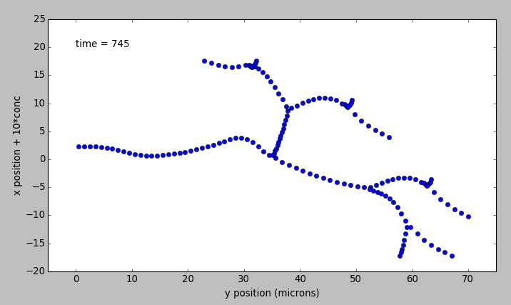
reacDiffBranchingNeuron.main()

This example illustrates how to define a kinetic model embedded in the branching pseudo 1-dimensional geometry of a neuron. This means that diffusion only happens along the axis of dendritic segments, not radially from inside to outside a dendrite, nor tangentially around the dendrite circumference. The model oscillates in space and time due to a Turing-like reaction-diffusion mechanism present in all compartments. For the sake of this demo, the initial conditions are set to be slightly different on one of the terminal dendrites, so as to break the symmetry and initiate oscillations. This example uses an external model file to specify a binary branching neuron. This model does not have any spines. The electrical model is used here purely for the geometry and is not part of the computations. In this example we build an identical chemical model throughout the neuronal geometry, using the makeChemModel function. The model is set up to run using the Ksolve for integration and the Dsolve for handling diffusion.

The display has two parts:

1. Animated pseudo-3D plot of neuronal geometry, where each point represents a diffusive voxel and moves in the y-axis to show changes in concentration.
2. Time-series plot that appears after the simulation has ended. The plots are for the first and last diffusive voxel, that is, the soma and the tip of one of the apical dendrites.

reacDiffBranchingNeuron.makeChemModel(compt)

This function sets up a simple oscillatory chemical system within the script. The reaction system is:

s ---a---> a  // s goes to a, catalyzed by a.
s ---a---> b  // s goes to b, catalyzed by a.
a ---b---> s  // a goes to s, catalyzed by b.
b -------> s  // b is degraded irreversibly to s.

in sum, a has a positive feedback onto itself and also forms b. b has a negative feedback onto a. Finally, the diffusion constant for a is 1/10 that of b.

reacDiffSpinyNeuron.main()

This example illustrates how to define a kinetic model embedded in the branching pseudo-1-dimensional geometry of a neuron. The model oscillates in space and time due to a Turing-like reaction-diffusion mechanism present in all compartments. For the sake of this demo, the initial conditions are set up slightly different on the PSD compartments, so as to break the symmetry and initiate oscillations in the spines. This example uses an external electrical model file with basal dendrite and three branches on the apical dendrite. One of those branches has a dozen or so spines. In this example we build an identical model in each compartment, using the makeChemModel function. One could readily define a system with distinct reactions in each compartment. The model is set up to run using the Ksolve for integration and the Dsolve for handling diffusion. The display has four parts:

1. animated line plot of concentration against main compartment#.
2. animated line plot of concentration against spine compartment#.
3. animated line plot of concentration against psd compartment#.
4. time-series plot that appears after the simulation has ended. The plot is for the last (rightmost) compartment.

reacDiffSpinyNeuron.makeChemModel(compt)

This function setus up a simple oscillatory chemical system within the script. The reaction system is:

s ---a---> a  // s goes to a, catalyzed by a.
s ---a---> b  // s goes to b, catalyzed by a.
a ---b---> s  // a goes to s, catalyzed by b.
b -------> s  // b is degraded irreversibly to s.

in sum, a has a positive feedback onto itself and also forms b. b has a negative feedback onto a. Finally, the diffusion constant for a is 1/10 that of b.

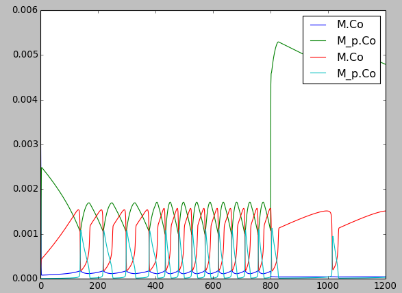
diffSpinyNeuron.main()

This example illustrates and tests diffusion embedded in the branching pseudo-1-dimensional geometry of a neuron. An input pattern of Ca stimulus is applied in a periodic manner both on the dendrite and on the PSDs of the 13 spines. The Ca levels in each of the dend, the spine head, and the spine PSD are monitored. Since the same molecule name is used for Ca in the three compartments, these are automagially connected up for diffusion. The simulation shows the outcome of this diffusion. This example uses an external electrical model file with basal dendrite and three branches on the apical dendrite. One of those branches has the 13 spines. The model is set up to run using the Ksolve for integration and the Dsolve for handling diffusion. The timesteps here are not the defaults. It turns out that the chem reactions and diffusion in this example are sufficiently fast that the chemDt has to be smaller than default. Note that this example uses rates quite close to those used in production models. The display has four parts:

1. animated line plot of concentration against main compartment#.
2. animated line plot of concentration against spine compartment#.
3. animated line plot of concentration against psd compartment#.
4. time-series plot that appears after the simulation has ended.

diffSpinyNeuron.makeChemModel(compt, doInput)

This function setus up a simple chemical system in which Ca input comes to the dend and to selected PSDs. There is diffusion between PSD and spine head, and between dend and spine head.

:: Ca_input ------> Ca // in dend and spine head only.

Manipulating Chemical Models

Running with different numerical methods

switchKineticSolvers.main()

At zero order, you can select the solver you want to use within the function moose.loadModel( filename, modelpath, solver ). Having loaded in the model, you can change the solver to use on it. This example illustrates how to assign and change solvers for a kinetic model. This process is necessary in two situations:

• If we want to change the numerical method employed, for example, from deterministic to stochastic.
• If we are already using a solver, and we have changed the reaction network by adding or removing molecules or reactions.

Note that we do not have to change the solvers if the volume or reaction rates change. In this example the model is loaded in with a gsl solver. The sequence of solver calculations is:

1. gsl
2. ee
3. gsl
4. gssa
5. gsl

If you're removing the solvers, you just delete the stoichiometry object and the associated ksolve/gsolve. Should there be diffusion (a dsolve)then you should delete that too. If you're building the solvers up again, then you must do the following steps in order:

1. build up the ksolve/gsolve and stoich (any order)
2. Assign stoich.ksolve
3. Assign stoich.path.

See the Reaction-diffusion section should you want to do diffusion as well.

Changing volumes

scaleVolumes.main()

This example illustrates how to run a model at different volumes. The key line is just to set the volume of the compartment:

compt.volume = vol

If everything else is set up correctly, then this change propagates through to all reactions molecules.

For a deterministic reaction one would not see any change in output concentrations. For a stochastic reaction illustrated here, one sees the level of 'noise' changing, even though the concentrations are similar up to a point. This example creates a bistable model having two enzymes and a reaction. One of the enzymes is autocatalytic. This model is set up within the script rather than using an external file. The model is set up to run using the GSSA (Gillespie Stocahstic systems algorithim) method in MOOSE.

To run the example, run the script

python scaleVolumes.py

and hit enter every cycle to see the outcome of stochastic calculations at ever smaller volumes, keeping concentrations the same.

Feeding tabulated input to a model

analogStimTable.analogStimTable()

Example of using a StimulusTable as an analog signal source in a reaction system. It could be used similarly to give other analog inputs to a model, such as a current or voltage clamp signal.

This demo creates a StimulusTable and assigns it half a sine wave. Then we assign the start time and period over which to emit the wave. The output of the StimTable is sent to a pool a, which participates in a trivial reaction:

table ----> a <===> b

The output of a and b are recorded in a regular table for plotting.

Finding steady states

This example sets up the kinetic solver and steady-state finder, on a bistable model of a chemical system. The model is set up within the script. The algorithm calls the steady-state finder 50 times with different (randomized) initial conditions, as follows:

• Set up the random initial condition that fits the conservation laws
• Run for 2 seconds. This should not be mathematically necessary, but for obscure numerical reasons it is much more likely that the steady state solver will succeed in finding a state.
• Find the fixed point
• Print out the fixed point vector and various diagnostics.
• Run for 10 seconds. This is completely unnecessary, and is done here just so that the resultant graph will show what kind of state has been found.

After it does all this, the program runs for 100 more seconds on the last found fixed point (which turns out to be a saddle node), then is hard-switched in the script to the first attractor basin from which it runs for another 100 seconds till it settles there, and then is hard-switched yet again to the second attractor and runs for 400 seconds.

Looking at the output you will see many features of note:

• the first attractor (stable point) and the saddle point (unstable fixed point) are both found quite often. But the second attractor is found just once. It has a very small basin of attraction.
• The values found for each of the fixed points match well with the values found by running the system to steady-state at the end.
• There are a large number of failures to find a fixed point. These are found and reported in the diagnostics. They show up on the plot as cases where the 10-second runs are not flat.

If you wanted to find fixed points in a production model, you would not need to do the 10-second runs, and you would need to eliminate the cases where the state-finder failed. Then you could identify the good points and keep track of how many of each were found.

There is no way to guarantee that all fixed points have been found using this algorithm! If there are points in an obscure corner of state space (as for the singleton second attractor convergence in this example) you may have to iterate very many times to find them.

You may wish to sample concentration space logarithmically rather than linearly.

findChemSteadyState.getState(ksolve, state)

This function finds a steady state starting from a random initial condition that is consistent with the stoichiometry rules and the original model concentrations.

findChemSteadyState.makeModel()

This function creates a bistable reaction system using explicit MOOSE calls rather than load from a file

Making a dose-response curve

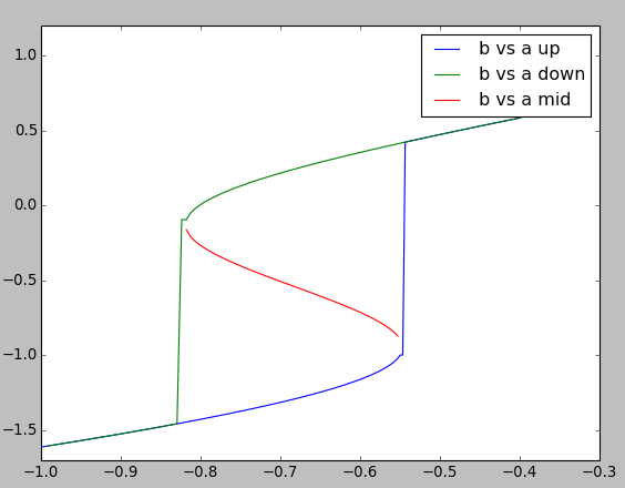
chemDoseResponse.main()

This example builds a dose-response of a bistable model of a chemical system. It uses the kinetic solver Ksolve and the steady-state finder SteadyState. The model is set up within the script.

The basic approach is to increment the control variable, a in this case, while monitoring b. The algorithm marches through a series of values of the buffered pool a and measures resultant values of pool b. At each cycle the algorithm calls the steady-state finder. Since a is incremented only a small amount on each step, each new steady state is (usually) quite close to the previous one. The exception is when there is a state transition.

Here we plot three dose-response curves to illustrate the bistable nature of the system.

On the upward going curve in blue, a starts low. Here, b follows the low arm of the curve and then jumps up to the high value at roughly log( [a] ) = -0.55.

On the downward going curve in green, b follows the high arm of the curve forming a nice hysteretic loop. Eventually b has to fall to the low state at about log( [a] ) = -0.83

Through nasty concentration manipulations, we find the third arm of the curve, which tracks the unstable fixed point. This is in red. We find this arm by setting an initial point close to the unstable fixed point, which the steady-state finder duly locates. We then follow a dose-response curve as with the other arms of the curve.

Note that the steady-state solver doesn't always succeed in finding a good solution, despite moving only in small steps. Nevertheless the resultant curves are smooth because it gives up pretty close to the correct value, simply because the successive points are close together. Overall, the system is pretty robust despite the core root-finder computations in GSL being temperamental.

In doing a production dose-response series you may wish to sample concentration space logarithmically rather than linearly.

chemDoseResponse.makeModel()

This function creates a bistable reaction system using explicit MOOSE calls rather than load from a file. The reaction is:

a ---b---> 2b    # b catalyzes a to form more of b.
2b ---c---> a    # c catalyzes b to form a.
a <======> 2b    # a interconverts to b.

Transport in branching dendritic tree

transportBranchingNeuron.main()

This example illustrates bidirectional transport embedded in the branching pseudo 1-dimensional geometry of a neuron. This means that diffusion and transport only happen along the axis of dendritic segments, not radially from inside to outside a dendrite, nor tangentially around the dendrite circumference. In this model there is a molecule a starting at the soma, which is transported out to the dendrites. There is another molecule, b, which is initially present at the dendrite tips, and is transported toward the soma. This example uses an external model file to specify a binary branching neuron. This model does not have any spines. The electrical model is used here purely for the geometry and is not part of the computations. In this example we build trival chemical model just having molecules a and b throughout the neuronal geometry, using the makeChemModel function. The model is set up to run using the Ksolve for integration and the Dsolve for handling diffusion.

The display has three parts:

1. Animated pseudo-3D plot of neuronal geometry, where each point represents a diffusive voxel and moves in the y-axis to show changes in concentration of molecule a.
2. Similar animated pseudo-3D plot for molecule b.
3. Time-series plot that appears after the simulation has ended. The plots are for the first and last diffusive voxel, that is, the soma and the tip of one of the apical dendrites.